Algorithms & Database for Graph Data

SC 4125: Developing Data Products

Module-5: Network Science Toolkit

by Anwitaman DATTA
School of Computer Science and Engineering, NTU Singapore.

Teaching material

• .html deck of slides
• .ipynb Jupyter notebook

Disclaimer/Caveat emptor

• Non-systematic and non-exhaustive review
• Illustrative approaches are not necessarily the most efficient or elegant, let alone unique

Acknowledgement & Disclaimer

The main narrative of this module is based on disparate sources. Parts of the content and codes are original, while others are based on 3rd party sources. I have attributed those sources to the best of my knowledge, and I have used those material following the principle of fair use.

Should anything in the material need to be changed or redacted, the copyright owners are requested to contact me at anwitaman@ntu.edu.sg

Connections matter!

Identify critical/important components: Supply chains, communication, transport, financial, crime networks, super-spreaders of an epidemic

Aviation network [Source: ICAO]

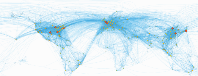
Identify communities: Groups and alliances, personalized recommendation, information spread and influence

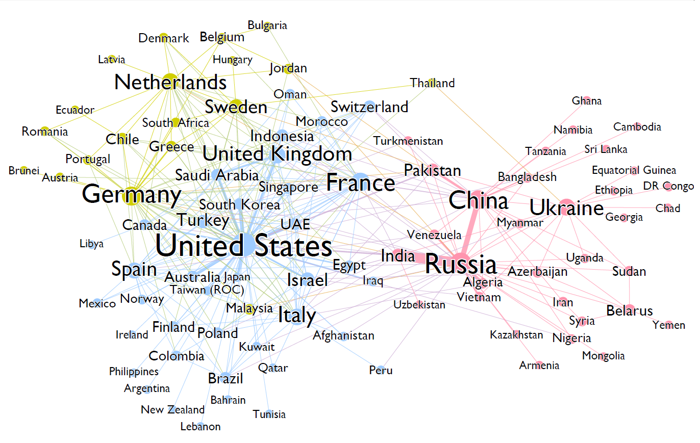
Arms trade network [Source: Algobeans.com]

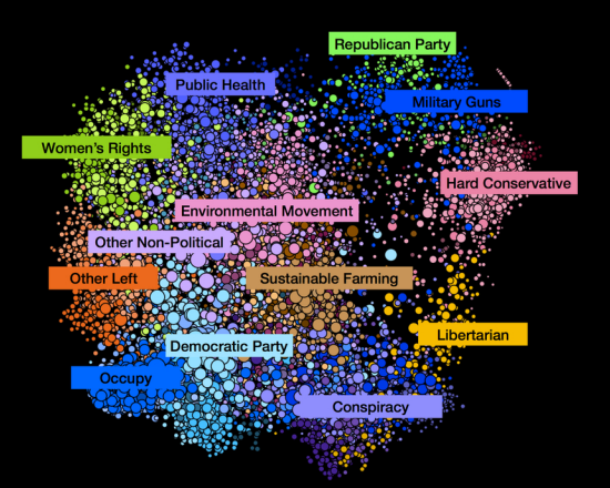
US Audience Groups on Facebook [Source: Social media polarization case-study]

Predicting relations

Determining transitive relations

9/11 hijackers network [Source: Terrorist network study]

Bitcoin flow trace [Source: Extortion case-study]

Module outline

Elementary concepts & definitions

Common graph algorithms & analysis techniques

NoSQL for graph data: Neo4j database & Cypher Query Language

Elementary concepts

# Some basic libraries
import networkx as nx
import matplotlib.pylab as plt
import pandas as pd

Types of graph

And how to realize them in NetworkX?

Types of graph: Undirected

nx.Graph()

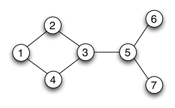
# Example - Undirected, unweigthed graph
UDG=nx.Graph()
UDG.add_edges_from([(1,2),(1,4),(2,3),(4,3),(3,5),(5,6),(5,7)])
# Individual edge can be added using add_edge
nx.draw(UDG, with_labels=True, node_color="silver")

# Example - Undirected, weighted graph
WG=nx.Graph()
WG.add_weighted_edges_from([(1,2,0.125),(1,3,0.75),(2,4,1.2),(3,4,0.375)])
            
list(WG.adjacency()) # Provides the adjacency list

[(1, {2: {'weight': 0.125}, 3: {'weight': 0.75}}),
 (2, {1: {'weight': 0.125}, 4: {'weight': 1.2}}),
 (3, {1: {'weight': 0.75}, 4: {'weight': 0.375}}),
 (4, {2: {'weight': 1.2}, 3: {'weight': 0.375}})]

# Example with a built-in graph
# Zachary's karate club: https://en.wikipedia.org/wiki/Zachary%27s_karate_club

G =  nx.karate_club_graph()
print('No of vertices: ',G.order())
print('No of edges: ',G.size())
pos = nx.spring_layout(G)
fig = plt.figure(figsize=(8,5))
nx.draw(G,pos, with_labels = 'true',node_color = 'gainsboro')
plt.show()

No of vertices:  34
No of edges:  78

for _ in G.adjacency():
    print(_)

(0, {1: {}, 2: {}, 3: {}, 4: {}, 5: {}, 6: {}, 7: {}, 8: {}, 10: {}, 11: {}, 12: {}, 13: {}, 17: {}, 19: {}, 21: {}, 31: {}})
(1, {0: {}, 2: {}, 3: {}, 7: {}, 13: {}, 17: {}, 19: {}, 21: {}, 30: {}})
(2, {0: {}, 1: {}, 3: {}, 7: {}, 8: {}, 9: {}, 13: {}, 27: {}, 28: {}, 32: {}})
(3, {0: {}, 1: {}, 2: {}, 7: {}, 12: {}, 13: {}})
(4, {0: {}, 6: {}, 10: {}})
(5, {0: {}, 6: {}, 10: {}, 16: {}})
(6, {0: {}, 4: {}, 5: {}, 16: {}})
(7, {0: {}, 1: {}, 2: {}, 3: {}})
(8, {0: {}, 2: {}, 30: {}, 32: {}, 33: {}})
(9, {2: {}, 33: {}})
(10, {0: {}, 4: {}, 5: {}})
(11, {0: {}})
(12, {0: {}, 3: {}})
(13, {0: {}, 1: {}, 2: {}, 3: {}, 33: {}})
(14, {32: {}, 33: {}})
(15, {32: {}, 33: {}})
(16, {5: {}, 6: {}})
(17, {0: {}, 1: {}})
(18, {32: {}, 33: {}})
(19, {0: {}, 1: {}, 33: {}})
(20, {32: {}, 33: {}})
(21, {0: {}, 1: {}})
(22, {32: {}, 33: {}})
(23, {25: {}, 27: {}, 29: {}, 32: {}, 33: {}})
(24, {25: {}, 27: {}, 31: {}})
(25, {23: {}, 24: {}, 31: {}})
(26, {29: {}, 33: {}})
(27, {2: {}, 23: {}, 24: {}, 33: {}})
(28, {2: {}, 31: {}, 33: {}})
(29, {23: {}, 26: {}, 32: {}, 33: {}})
(30, {1: {}, 8: {}, 32: {}, 33: {}})
(31, {0: {}, 24: {}, 25: {}, 28: {}, 32: {}, 33: {}})
(32, {2: {}, 8: {}, 14: {}, 15: {}, 18: {}, 20: {}, 22: {}, 23: {}, 29: {}, 30: {}, 31: {}, 33: {}})
(33, {8: {}, 9: {}, 13: {}, 14: {}, 15: {}, 18: {}, 19: {}, 20: {}, 22: {}, 23: {}, 26: {}, 27: {}, 28: {}, 29: {}, 30: {}, 31: {}, 32: {}})

for _ in nx.generate_adjlist(G):
    print(_)

0 1 2 3 4 5 6 7 8 10 11 12 13 17 19 21 31
1 2 3 7 13 17 19 21 30
2 3 7 8 9 13 27 28 32
3 7 12 13
4 6 10
5 6 10 16
6 16
7
8 30 32 33
9 33
10
11
12
13 33
14 32 33
15 32 33
16
17
18 32 33
19 33
20 32 33
21
22 32 33
23 25 27 29 32 33
24 25 27 31
25 31
26 29 33
27 33
28 31 33
29 32 33
30 32 33
31 32 33
32 33
33

nx.adjacency_matrix(G)

<34x34 sparse matrix of type '<class 'numpy.intc'>'
	with 156 stored elements in Compressed Sparse Row format>

# Visualizing the (sparse) adjacency matrix
plt.spy(nx.adjacency_matrix(G), c='gainsboro')

<matplotlib.lines.Line2D at 0x22a4a2f6370>

Types of graph: Directed

nx.DiGraph()

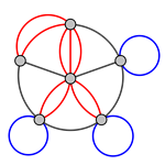
Types of graph: Multigraph

Graphs with self loops and parallel edges

nx.MultiGraph()
nx.MultiDiGraph()

Types of graph: Multi-mode

Graphs with multiple kinds of nodes

Use node attribute

G.add_node(1, attr_name=“XXX")

Types of graph: Bipartite

Graphs with two disjoint sets of nodes, where no two nodes within a given set are adjacent

Determine if a graph is bipartite using is_bipartite()

Network properties & models

Scale-free networks: degree distribution follows a power law

i.e., $P(k) \sim k^{\gamma}$ where $\gamma$ is the scaling parameter (with typical value between 2 and 3)

• Models & network formation hypothesis
  • Small-world phenomenon
  • Preferential attachment

Ungraded Task 5.1

Determine the distribution of pair-wise shortest path lengths, and the diameter of the Karate club graph.

Here's one way to solve this: try it yourself first, though!. In the link, you will also find how a few other distance measures are computed.

Algorithms & analysis

Scope: Not the algorithmic intricacies. Our emphasis here is more on understanding them at an intuitive level - "what do they do/don't do?" and "when/how to use them?".

Centrality

• Identify important vertices
  • Discuss: What determines importance though?
    • Variation: Identify important links

# Degree centrality
# The degree centrality for a node v is the fraction of nodes it is connected to

cD = nx.degree_centrality(G)
print(cD)

{0: 0.48484848484848486, 1: 0.2727272727272727, 2: 0.30303030303030304, 3: 0.18181818181818182, 4: 0.09090909090909091, 5: 0.12121212121212122, 6: 0.12121212121212122, 7: 0.12121212121212122, 8: 0.15151515151515152, 9: 0.06060606060606061, 10: 0.09090909090909091, 11: 0.030303030303030304, 12: 0.06060606060606061, 13: 0.15151515151515152, 14: 0.06060606060606061, 15: 0.06060606060606061, 16: 0.06060606060606061, 17: 0.06060606060606061, 18: 0.06060606060606061, 19: 0.09090909090909091, 20: 0.06060606060606061, 21: 0.06060606060606061, 22: 0.06060606060606061, 23: 0.15151515151515152, 24: 0.09090909090909091, 25: 0.09090909090909091, 26: 0.06060606060606061, 27: 0.12121212121212122, 28: 0.09090909090909091, 29: 0.12121212121212122, 30: 0.12121212121212122, 31: 0.18181818181818182, 32: 0.36363636363636365, 33: 0.5151515151515151}

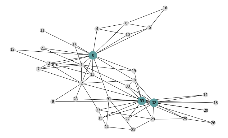
Top 3 degree-central nodes highlighted

A few frequently used centrality measures

• Betweenness centrality: nx.betweenness_centrality(G)

  Betweenness centrality of a node $v$ is the sum of the fraction of all-pairs shortest paths that pass through $v$

  • Variation: edge_betweenness_centrality to determine important edges

• Closeness centrality: nx.closeness_centrality(G)

  Closeness centrality of a node $v$ is the reciprocal of the average shortest path distance to $v$ over all n-1 reachable nodes.

• Katz centrality: nx.katz_centrality(G)

  Katz centrality computes the centrality for a node based on the centrality of its neighbors. It is a generalization of the eigenvector centrality.

Many other centrality measures exist. List of the ones available with NetworkX.

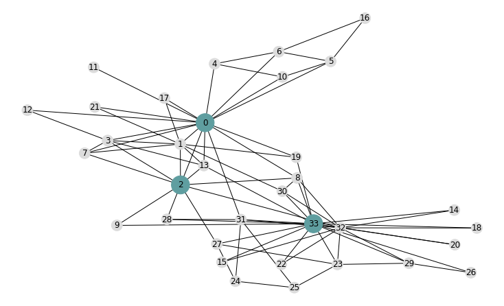
Top-3 closeness central nodes highlighted

Ungraded Task 5.2:

Ungraded Task 5.2.1: Draw the Karate club graph, highlighting top-K central nodes (using a centrality measure of your choice).

Ungraded Task 5.2.2: Rank the node centralities using different algorithms (e.g., the few mentioned above), and determine which of these algorithms yield similar and the most distinct results (for the Karate club graph).

Community detection (graph clustering)

What determines communities in a network?

• partitions, hierarchies, fuzzy communities

Modularity

Modularity is the fraction of the edges that fall within the given groups minus the expected fraction if edges were distributed at random.

Image source: Neo4j.com

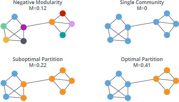
c = list(nx.algorithms.community.greedy_modularity_communities(G))
# An alternate (more popular) modularity optimization algorithm is Louvain algorithm
# Louvain is currently not implemented in NetworkX. You may access it by installing python-louvain
colors = []
for node in G:
    for i in range(len(c)):
        if node in c[i]:
            colors.append(i)
            
fig = plt.figure(figsize=(8,4.5))        
nx.draw(G,pos, with_labels = 'true',cmap=plt.cm.Paired, node_color=colors)
plt.show()

K-cliques

A k-clique community is the union of all cliques of size k that can be reached through adjacent (sharing k-1 nodes) k-cliques.

• Analyst has to choose k (meaningfully)

c = list(nx.algorithms.community.k_clique_communities(G,3))
# This again produces three groups (but some nodes are not included in any of these groups)
# While some of these groups are overlapping
print(c)
print(c[0].intersection(c[1]))

[frozenset({0, 1, 2, 3, 7, 8, 12, 13, 14, 15, 17, 18, 19, 20, 21, 22, 23, 26, 27, 28, 29, 30, 31, 32, 33}), frozenset({0, 4, 5, 6, 10, 16}), frozenset({24, 25, 31})]
frozenset({0})

Label propagation

1. Every node is initialized with a (unique) label.
2. The labels propagate through the network iteratively: Each node updates its label to the one that the maximum number of its neighbors have (peer pressure ;).
   • Ties are broken uniformly and randomly.

p.s. Easy to parallelize and distribute the computation

c = list(nx.algorithms.community.label_propagation_communities(G))
colorsLP = []
for node in G:
    for i in range(len(c)):
        if node in c[i]:
            colorsLP.append(i)
            
fig = plt.figure(figsize=(8,4.5))        
nx.draw(G,pos, with_labels = 'true',cmap=plt.cm.Paired, node_color=colorsLP)
plt.show()

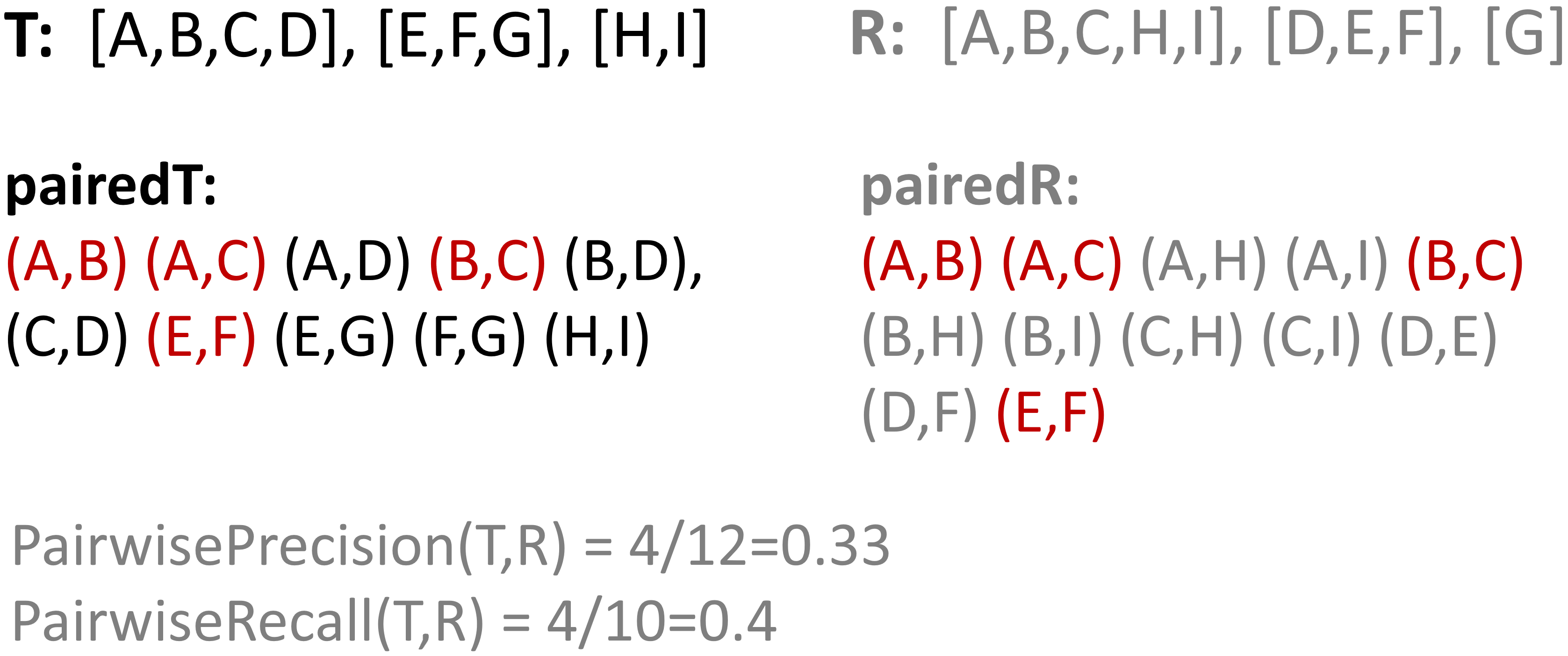
Metrics for comparing communities?

• One popular measure: Pairwise F1-measure
  • For a given result $R$ and a given truth/baseline $T$:
    • $PairwisePrecision(T,R)=\frac{|pairedR \space \cap \space pairedT|}{|pairedR|}$
      • fraction of reference pairs in the result R that are also in the truth T
    • $PairwiseRecall(T,R)=\frac{|pairedR \space \cap \space pairedT|}{|pairedT|}$
      • fraction of reference pairs in the truth T that are also in the result R
    • $Pairwise \space F_1 = 2 \times \frac{PairwisePrecision \times PairwiseRecall}{PairwisePrecision + PairwiseRecall}$
      • Harmonic mean (a weighted variation exists, called $F_{\beta}$)
• See Evaluation of Clusterings -- Metrics and Visual Support by Achtert et al. for more discussions on comparing clustering results.

Ungraded Task 5.3

Compute the F1 score between the communities determined using modularity and label propagation methods.

• Note that one of the limitations of F1 score is that it is unsuitable for fuzzy communities where same node may belong to multiple communities.

Link prediction

Predicting the existence/creation of a link between two entities in a network

Based on common neighbors

• Underlying idea: Triadic closure
  • Number of common neighbors
  • Jaccard coefficient: Number of common neighbors normalized by total number of neighbors
    • $\frac{\Gamma(u) \cap \Gamma(v)}{\Gamma(u) \cup \Gamma(v)}$ where $\Gamma(x)$ is the set of neighbors of node $x$

# Common neighbors
# list node pairs which are not already neighbors
# ordered in decreasing number of common neighbors
topK=20
comm_neigh = [(e[0],e[1], len(list(nx.common_neighbors(G,e[0],e[1])))) for e in nx.non_edges(G)]
sortedCN = sorted(comm_neigh, key=lambda kv: kv[2],reverse=True)
print(sortedCN[0:topK])

[(2, 33, 6), (0, 33, 4), (7, 13, 4), (0, 32, 3), (1, 8, 3), (1, 33, 3), (2, 30, 3), (2, 31, 3), (4, 5, 3), (6, 10, 3), (8, 13, 3), (8, 31, 3), (13, 19, 3), (23, 31, 3), (27, 32, 3), (28, 32, 3), (0, 16, 2), (0, 28, 2), (0, 30, 2), (1, 12, 2)]

# Jaccard coefficient
jac_coeffs = list(nx.jaccard_coefficient(G))
# Notice that it transparently determines non-edges
sortedJC= sorted(jac_coeffs, key=lambda kv: kv[2],reverse=True)
print(sortedJC[0:topK])

[(14, 15, 1.0), (14, 18, 1.0), (14, 20, 1.0), (14, 22, 1.0), (15, 18, 1.0), (15, 20, 1.0), (15, 22, 1.0), (17, 21, 1.0), (18, 20, 1.0), (18, 22, 1.0), (20, 22, 1.0), (7, 13, 0.8), (4, 5, 0.75), (6, 10, 0.75), (9, 28, 0.6666666666666666), (17, 19, 0.6666666666666666), (19, 21, 0.6666666666666666), (13, 19, 0.6), (7, 12, 0.5), (7, 17, 0.5)]

# If we want to compute the score for specific (set of) node pairs, that too can be done 
# Example: nx.jaccard_coefficient(G, [(0, 1), (2, 3)])
list(nx.jaccard_coefficient(G, [(0, 1),(6, 16)]))
# Naturally, you can also compute this for node pairs which are adjacent, e.g., 6 and 16

[(0, 1, 0.3888888888888889), (6, 16, 0.2)]

Based on nodes' importances to their common neighbors individually

• Underlying idea: How spread/concentrated are the ties
  • Resource allocation
  • Adamic-Adar

# Resource Allocation
res_alloc = list(nx.resource_allocation_index(G))
sortedRA= sorted(res_alloc, key=lambda kv: kv[2],reverse=True)
print(sortedRA[0:topK])

[(2, 33, 1.5666666666666664), (0, 33, 0.9), (1, 33, 0.7833333333333333), (4, 5, 0.6458333333333333), (6, 10, 0.6458333333333333), (23, 24, 0.5833333333333333), (25, 27, 0.5333333333333333), (0, 16, 0.5), (2, 31, 0.47916666666666663), (23, 31, 0.47549019607843135), (0, 32, 0.4666666666666667), (7, 13, 0.44027777777777777), (24, 33, 0.41666666666666663), (1, 8, 0.4125), (2, 30, 0.39444444444444443), (27, 31, 0.39215686274509803), (25, 32, 0.3666666666666667), (25, 33, 0.3666666666666667), (27, 32, 0.35882352941176476), (1, 32, 0.35)]

# Adamic-Adar index
AdAd = list(nx.adamic_adar_index(G))
sortedAA= sorted(AdAd, key=lambda kv: kv[2],reverse=True)
print(sortedAA[0:topK])

[(2, 33, 4.719381261461351), (0, 33, 2.7110197222973085), (1, 33, 2.252921681630931), (4, 5, 1.9922605072935597), (6, 10, 1.9922605072935597), (7, 13, 1.8081984819901584), (2, 31, 1.6733425912309228), (23, 31, 1.6656249548734432), (23, 24, 1.631586747071319), (0, 32, 1.613740043014111), (25, 27, 1.531574161186449), (1, 8, 1.5163157625699744), (2, 30, 1.4788841522548752), (0, 16, 1.4426950408889634), (27, 32, 1.4085855403276248), (28, 32, 1.34536123231926), (24, 33, 1.279458146995729), (27, 31, 1.2631953504915985), (25, 32, 1.179445561110859), (25, 33, 1.179445561110859)]

Preferential attachment

• Underlying idea: More popular nodes are likely "target of choice" to connect with
  • NetworkX implementation uses $|\Gamma(u)|\times|\Gamma(v)|$ to determine preferential attachment score between nodes $u$ and $v$.
    • This is essentially the product of their degree centralities
    • Some other centrality scores too could be used instead

pref_at = nx.preferential_attachment(G)
sortedPA= sorted(pref_at, key=lambda kv: kv[2],reverse=True)
print(sortedPA[0:topK])

[(0, 33, 272), (0, 32, 192), (2, 33, 170), (1, 33, 153), (1, 32, 108), (3, 33, 102), (0, 23, 80), (3, 32, 72), (5, 33, 68), (6, 33, 68), (7, 33, 68), (0, 27, 64), (0, 29, 64), (0, 30, 64), (2, 31, 60), (13, 32, 60), (1, 31, 54), (4, 33, 51), (10, 33, 51), (24, 33, 51)]

Using community information/side information

• Underlying idea: Being part of a common community increases chance of linking up
  • Soundarajan Hopcroft
    • Variations: based on common neighbour count and resource allocation
  • Within inter-cluster
    • Compute the ratio of within- and inter-cluster common neighbors

# I am using the partitions created previosuly from Label Propagation algorithm
for node in G:
    G.nodes[node]["community"] = colorsLP[node] 

SH_cn_coeff = nx.cn_soundarajan_hopcroft(G,community='community')
sortedSHcn=sorted(SH_cn_coeff, key=lambda kv: kv[2],reverse=True)
SH_ra_coeff = nx.ra_index_soundarajan_hopcroft(G,community='community')
sortedSHra=sorted(SH_ra_coeff, key=lambda kv: kv[2],reverse=True)
#preds.sort(key = operator.itemgetter(2),reverse=True)
print(sortedSHcn[0:topK])
print()
print(sortedSHra[0:topK])

[(2, 33, 11), (7, 13, 7), (27, 32, 6), (2, 30, 5), (13, 19, 5), (28, 32, 5), (0, 33, 4), (1, 12, 4), (2, 23, 4), (3, 17, 4), (3, 19, 4), (3, 21, 4), (7, 12, 4), (7, 17, 4), (7, 19, 4), (7, 21, 4), (8, 9, 4), (8, 14, 4), (8, 15, 4), (8, 18, 4)]

[(2, 33, 1.3666666666666665), (27, 32, 0.35882352941176476), (7, 13, 0.3402777777777778), (2, 23, 0.3333333333333333), (23, 26, 0.3088235294117647), (26, 32, 0.3088235294117647), (2, 30, 0.2833333333333333), (27, 29, 0.25882352941176473), (1, 12, 0.22916666666666666), (7, 12, 0.22916666666666666), (12, 13, 0.22916666666666666), (3, 17, 0.1736111111111111), (3, 19, 0.1736111111111111), (3, 21, 0.1736111111111111), (7, 17, 0.1736111111111111), (7, 19, 0.1736111111111111), (7, 21, 0.1736111111111111), (13, 17, 0.1736111111111111), (13, 19, 0.1736111111111111), (13, 21, 0.1736111111111111)]

IntClust_coeff=nx.within_inter_cluster(G, delta=0.001, community='community')
sortedIC=sorted(IntClust_coeff, key=lambda kv: kv[2],reverse=True)
print(sortedIC[0:topK]) 

[(27, 32, 3000.0), (1, 12, 2000.0), (2, 23, 2000.0), (3, 17, 2000.0), (3, 19, 2000.0), (3, 21, 2000.0), (7, 12, 2000.0), (7, 17, 2000.0), (7, 19, 2000.0), (7, 21, 2000.0), (8, 9, 2000.0), (8, 14, 2000.0), (8, 15, 2000.0), (8, 18, 2000.0), (8, 20, 2000.0), (8, 22, 2000.0), (8, 23, 2000.0), (8, 27, 2000.0), (8, 28, 2000.0), (8, 29, 2000.0)]

Ungraded Task 5.4

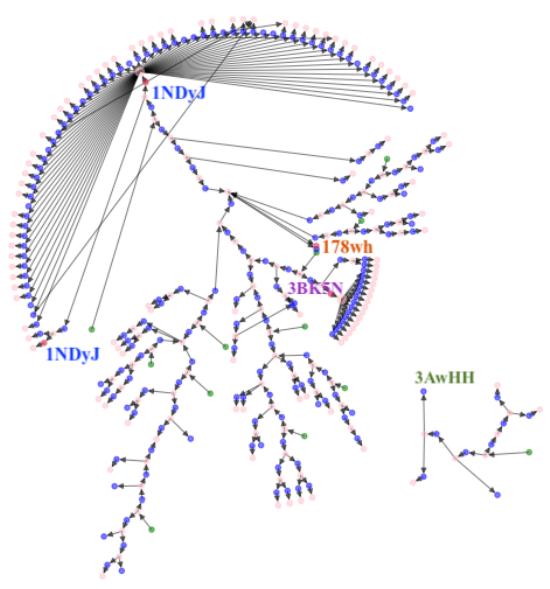
• Consider the HPD graph data provided in the HPD_full.net file
  • Obtained from https://noesis.ikor.org/datasets/link-prediction
• Consider an simple version of the graph
  • if needed, remove directionality, self-loops and multiple edges between any specific node pairs
• For the resulting graph, divide (randomly) ~90% edges to "train" your link predictor. Use ~10% edges to "validate" your predictions.
  • You may want to use a seed for randomness, so that your experiments are reproducible
• Ungraded Task 5.4.1: Apply individually some of the basic link prediction approaches available in NetworkX, consider the top candidates (equal to the validation set size) to determine Recall and Precision of prediction per approach.
• Ungraded Task 5.4.2: Use the individual measures as features and apply machine learning technique(s) of your choice, to predict links. Report Recall, Precision (and any other metrics of interest) to determine the quality of your prediction.
  • Make sure that you use the same 10% for comparison across subtasks.
    • Though you may repeat the exercise with different subsets to study in/consistency.

# To get you started: NetworkX has support to read several data formats 
HPD_gr = nx.read_pajek("data/HPD_full.net") # change path as suitable
HPD_ugr=nx.to_undirected(HPD_gr)
print(len(HPD_gr.nodes()),len(HPD_gr.edges()))

8756 32331

Neo4j

and Cypher

The following content on Neo4j and Cypher is (primarily) based on the book Graph Databases by Robinson et al. (specifically Chapter 3, where Cypher is discussed), and documentation resources on Neo4j website. Unless a different source is stated, the image snippets used in the following are from the stated book and Neo4j website. Neo4j provides for free this book as well as several other books on Graph DB, Algorithms and Data Science. Memgraph.com has a nice cheat sheet to get basic familiarity quickly with Cypher.

Why Neo4j?

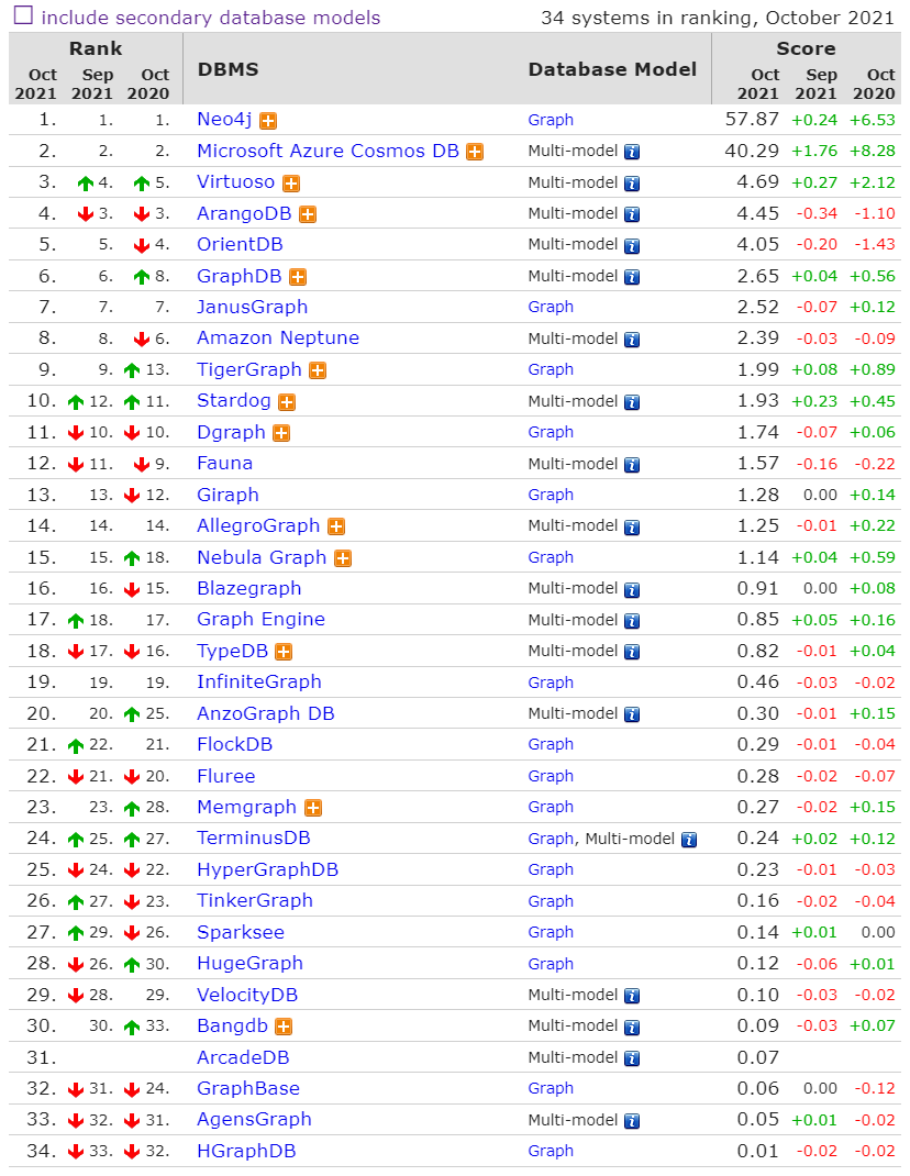
Source: db-engines.com

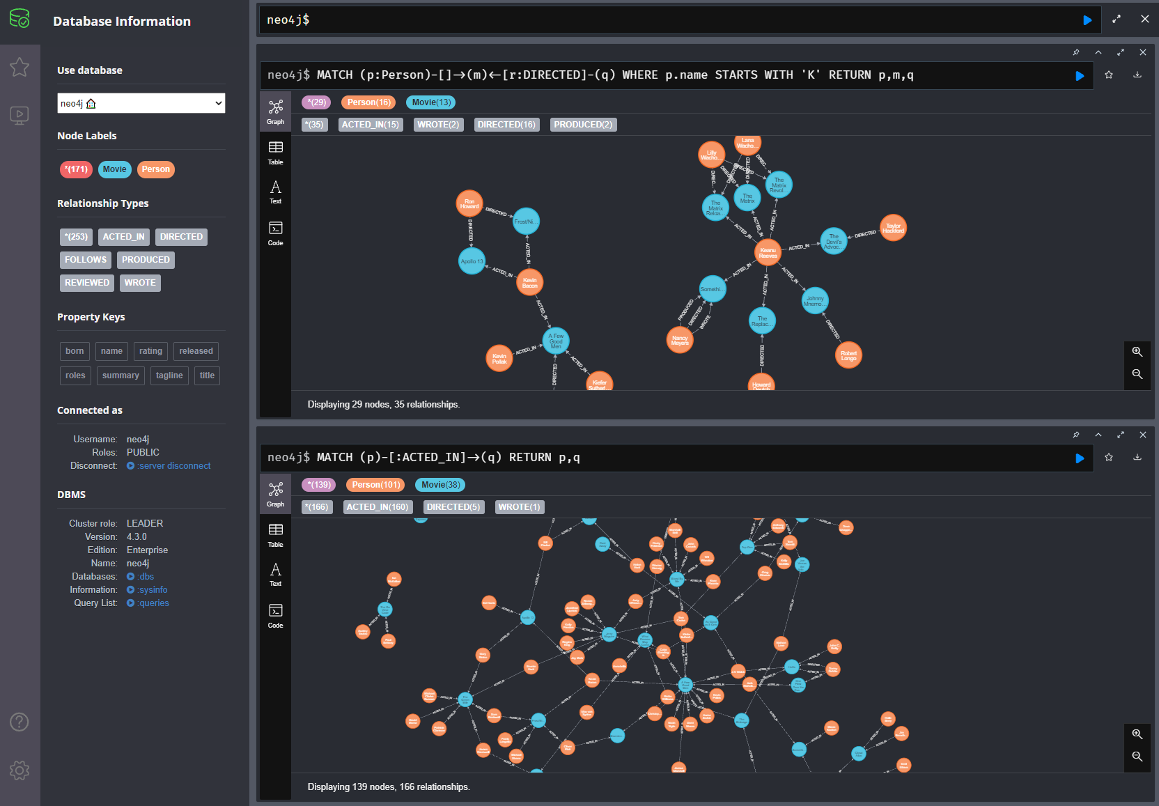
Neo4j/Aura interface

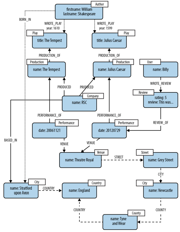
Data model

• nodes
  • properties: Nodes contain properties in the form of arbitrary key-value pairs.
  • labels: Tags for the nodes, indicating role(s) the nodes play.
• relationships: A relationship in Neo4j is directed, with a start node and end node and a single name.
  • properties: Similar to nodes, relationships can also have properties.

Example

Flexibility Accommodate multiple domains together: Literary domain (authors, works, etc), Theatrical domain (productions, performances, reviews, etc), Geospatial data Consider and contrast modeling this data using traditional RDBMS: Freedom from managing foreign keys, expensive joins! Organically update "schema" by gradually adding more kinds of nodes or relationships

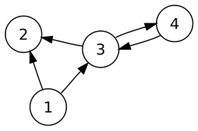
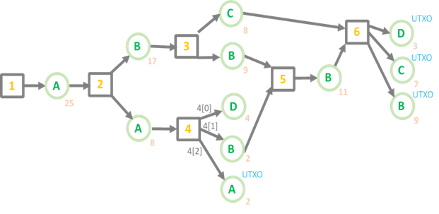
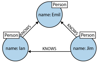
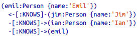
Cypher's ASCII pattern based declarative representation

Graph structure

• (emil)<-[:KNOWS]-(jim)-[:KNOWS]->(ian)-[:KNOWS]->(emil)
• (e)<-[:KNOWS]-(j)-[:KNOWS]->(i)-[:KNOWS]->(e)

• Identifiers: Allow reference to the same node more than once when describing a pattern.
  • Query description with only one dimension (text proceeding from left to right) is able to capture a graph laid out in two dimensions.
  • Cypher patterns follow very naturally from the way we draw the graph.

Binding the pattern to specific data instances

• specify some property values and node labels that help locate the relevant elements in the dataset

Match and Return

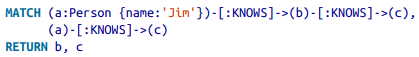
• nodes are written inside parenthesis ()
  • node labels are prefixed by colons, e.g., :Person
  • the identifiers, e.g., a, b and c are on the left of the colon
    • use of identifier is optional: used if one needs to reference back to it
• nodes can be anonymous in the query: e.g, (theater)<-[:VENUE]-()
  • relationships are written as --> OR <-- indicating directions
  • relationship names are indicated between the dashes, encapslated by square brackets, and prefixed by colon, e.g. -[:KNOWS]-
  • relationships or nodes may also be unnamed

• curly braces are used to indicate node and relationship propery key-value pairs, e.g., {name:'Jim'}
  • in the example query, providing such a specific value creates an anchor in the graph, tying the query to a specific (set of) node instance(s)
  • underlying indexing helps optimize the search of the instances
    • one can explicitly ask to create indices also with
      CREATE INDEX ON :LabelName(PropertyName)
  • one can explicitly put in certain constraints also, e.g. Node property uniqueness (which is automatically indexed)
    • some constraints are exclusive to the Enterprise edition: See more on constraints

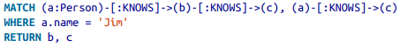
Match, Where and Return

Alternate expression of the same query, using WHERE for anchoring

WHERE clause can more generally be used to describe constrains on match

• e.g, WHERE p.born <= 1940

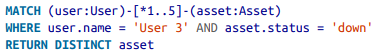
Indeterminate paths

Queries with indeterminate relationships - both in terms of types, and distance within the graph can be composed.

Check the book & manual for numerous other Cypher options and features

• Post-processing results: aggregation, ordering, filtering, etc.
• Query chaining (writing complex queries in simplers sub-parts)
• Common data modelling pitfalls
• Loading and modifying data
  • Cypher instructions, e.g. CREATE
  • Bulk data uplaod
    • Import .csv files
    • neo4j-admin import tool
• Database management, access control, etc.

Hands-on with Neo4j and Cypher

I use Neo4j's cloud service Aura along with its default Movie data set for the demo codes that follow.

The example code snippets used here are based on and expands over Neo4j's introduction to Cypher and a nice and short Medium article on how to integrate Neo4j with Jupyter notebook, which use the same movie dataset.

#!pip install neo4j
#!pip install neo4j-driver==1.6.2
#!pip install --upgrade py2neo==2021.1.5 
## The latter version (2021.2.0) of py2neo unfortunately triggers errors with rest of my environment setup
## To use this code with rest of your config, you may have to play around with the neo4j driver and py2neo versions 
# You may also need to restrat kernel after installations
import neo4j
from py2neo import Graph,Node,Relationship,NodeMatcher 
# Also checkout https://pypi.org/project/ipython-cypher/ for using Cypher with Jupyter magic
## I have worked with it with local DB instance, however I could not make it work with Aura and my current configurations

# DB credentials obfuscated: Replace this portion with your own credentials
# Comment the following out, and populate your own 
fo = open("neo4j-Aura-creds.txt", "r")
strng = fo.readlines()
fo.close()

URI=strng[0].strip()
UserID=strng[1].strip()
NeoPass=strng[2].strip()

# Uncomment and populate your info based on your own instance, replacing the XXX
# URI="XXX"
# UserID="XXX"
# NeoPass="XXX"

# Connect to the Neo4j server 
# URI could be as from the Aura cloud service, or your local instance
# For exposition, I am using Aura, along with the default "Movie database" 
# My URI looks like: neo4j+s://XXX.databases.neo4j.io

graph = Graph(URI, auth=(UserID, NeoPass))

The Movie dataset

Default dataset with Aura

# What kinds of nodes are there in the DB?

nodetype_query="MATCH (n) RETURN DISTINCT labels(n) as NodeType"
nodetype_result=graph.run(nodetype_query).to_data_frame()
nodetype_result

	NodeType
0	[Movie]
1	[Person]

# What kinds of properties do the nodes have?

MovieProperty="MATCH (n) RETURN DISTINCT labels(n) as NodeType, keys(n) as Properties ORDER BY labels(n)"
Movie_pro_result=graph.run(MovieProperty).to_data_frame()
Movie_pro_result

	NodeType	Properties
0	[Movie]	[tagline, title, released]
1	[Movie]	[title, released, tagline]
2	[Movie]	[released, tagline, title]
3	[Movie]	[title, released]
4	[Person]	[name, born]
5	[Person]	[name]

# What kinds of relationships are there in the DB?
cypher_all_relationship="MATCH (n)-[r]-(m) RETURN DISTINCT type(r) as RelationType, keys(r) as Properties"
graph.run(cypher_all_relationship).to_data_frame()

	RelationType	Properties
0	ACTED_IN	[roles]
1	PRODUCED	[]
2	DIRECTED	[]
3	WROTE	[]
4	REVIEWED	[summary, rating]
5	REVIEWED	[rating, summary]
6	FOLLOWS	[]

# Aggregation query example
number_of_person_nodes="MATCH(p:Person) RETURN Count(p)"
number_of_movie_nodes="MATCH(m:Movie) RETURN Count(m)"

#Evaluate the Cypher query
result_persons=graph.evaluate(number_of_person_nodes)
result_movies=graph.evaluate(number_of_movie_nodes)

#Print the result
print(f" No of person nodes: {result_persons} \n No of movie nodes: {result_movies}")

 No of person nodes: 133 
 No of movie nodes: 38

#Cypher to fetch the actors along with the movies they acted in
actors_movies="MATCH (p:Person)-[rel:ACTED_IN]->(m:Movie) RETURN DISTINCT p.name as PersonName,m.title as MovieName ORDER BY PersonName ASC"
act_movie_df=graph.run(actors_movies).to_data_frame()
act_movie_df

	PersonName	MovieName
0	Aaron Sorkin	A Few Good Men
1	Al Pacino	The Devil's Advocate
2	Annabella Sciorra	What Dreams May Come
3	Anthony Edwards	Top Gun
4	Audrey Tautou	The Da Vinci Code
...	...	...
167	Victor Garber	Sleepless in Seattle
168	Werner Herzog	What Dreams May Come
169	Wil Wheaton	Stand By Me
170	Zach Grenier	RescueDawn
171	Zach Grenier	Twister

172 rows × 2 columns

#Query to fetch people who have worked alongside Kevin Bacon in any movie (any kind of relationship) 
colleagues_name="MATCH (p:Person {name:'Kevin Bacon'})-[*2..2]-(c:Person) RETURN DISTINCT p.name as PersonName,c.name as Colleague ORDER BY Colleague ASC"
# Note: If we want to find only people who have acted alongside Kevin Bacon, the query needs to be modified
coll_df=graph.run(colleagues_name).to_data_frame()
coll_df

	PersonName	Colleague
0	Kevin Bacon	Aaron Sorkin
1	Kevin Bacon	Bill Paxton
2	Kevin Bacon	Christopher Guest
3	Kevin Bacon	Cuba Gooding Jr.
4	Kevin Bacon	Demi Moore
5	Kevin Bacon	Ed Harris
6	Kevin Bacon	Frank Langella
7	Kevin Bacon	Gary Sinise
8	Kevin Bacon	J.T. Walsh
9	Kevin Bacon	Jack Nicholson
10	Kevin Bacon	James Marshall
11	Kevin Bacon	Kevin Pollak
12	Kevin Bacon	Kiefer Sutherland
13	Kevin Bacon	Michael Sheen
14	Kevin Bacon	Noah Wyle
15	Kevin Bacon	Oliver Platt
16	Kevin Bacon	Rob Reiner
17	Kevin Bacon	Ron Howard
18	Kevin Bacon	Sam Rockwell
19	Kevin Bacon	Tom Cruise
20	Kevin Bacon	Tom Hanks

#Query to fetch co-actors of Kevin Bacon
coact_name="MATCH (p:Person {name:'Kevin Bacon'})-[:ACTED_IN*2..2]-(c:Person) RETURN DISTINCT p.name as PersonName,c.name as CoActor ORDER BY CoActor ASC"
# Note: If we want to find only people who have acted alongside Kevin Bacon, the query needs to be modified
coact_df=graph.run(coact_name).to_data_frame()
coact_df

	PersonName	CoActor
0	Kevin Bacon	Aaron Sorkin
1	Kevin Bacon	Bill Paxton
2	Kevin Bacon	Christopher Guest
3	Kevin Bacon	Cuba Gooding Jr.
4	Kevin Bacon	Demi Moore
5	Kevin Bacon	Ed Harris
6	Kevin Bacon	Frank Langella
7	Kevin Bacon	Gary Sinise
8	Kevin Bacon	J.T. Walsh
9	Kevin Bacon	Jack Nicholson
10	Kevin Bacon	James Marshall
11	Kevin Bacon	Kevin Pollak
12	Kevin Bacon	Kiefer Sutherland
13	Kevin Bacon	Michael Sheen
14	Kevin Bacon	Noah Wyle
15	Kevin Bacon	Oliver Platt
16	Kevin Bacon	Sam Rockwell
17	Kevin Bacon	Tom Cruise
18	Kevin Bacon	Tom Hanks

#Query to fetch people who have worked alongside Kevin Bacon in any movie (but they were not co-actors) 
# Using WHERE clause of the form (NOT X) OR (NOT Y)
colleagues_notcoactors_name="MATCH (p:Person {name:'Kevin Bacon'})-[*2..2]-(c:Person) WHERE  (NOT (p)--()-[:ACTED_IN]-(c)) OR (NOT (p)-[:ACTED_IN]-()--(c)) RETURN DISTINCT p.name as PersonName,c.name as Colleague ORDER BY Colleague ASC"
notcoact_df=graph.run(colleagues_notcoactors_name).to_data_frame()
notcoact_df

	PersonName	Colleague
0	Kevin Bacon	Rob Reiner
1	Kevin Bacon	Ron Howard

#Query to fetch people who have worked alongside Kevin Bacon in any movie (but they were not co-actors) 
# Using alternate, slightly simplified formulation leveraging (NOT X) OR (NOT Y) = NOT (X AND Y) 
colleagues_notcoactors_name="MATCH (p:Person {name:'Kevin Bacon'})-[*2..2]-(c:Person) WHERE NOT ( (p)--()-[:ACTED_IN]-(c) AND (p)-[:ACTED_IN]-()--(c)) RETURN DISTINCT p.name as PersonName,c.name as Colleague ORDER BY Colleague ASC"
notcoact_df=graph.run(colleagues_notcoactors_name).to_data_frame()
notcoact_df

	PersonName	Colleague
0	Kevin Bacon	Rob Reiner
1	Kevin Bacon	Ron Howard

# What was the nature of thier relationships in these cases?
for x in notcoact_df['Colleague']:
    rob_relationship="MATCH (p:Person {name:'Kevin Bacon'})-[r1]-(m)-[r2]-(q:Person {name:'" + x + "'}) RETURN DISTINCT type(r1), type(r2), m.title"
    rel_data=graph.run(rob_relationship).data()
    print('Kevin Bacon ' + rel_data[0]['type(r1)'] + ' and ' + x + " " + rel_data[0]['type(r2)'] + " the movie " +rel_data[0]['m.title'])

Kevin Bacon ACTED_IN and Rob Reiner DIRECTED the movie A Few Good Men
Kevin Bacon ACTED_IN and Ron Howard DIRECTED the movie Apollo 13

py2neo's native matching

py2neo provides certain functionality that can be used "bypassing" writing your own Cyper query See py2neo documentation for details. The code snippets are based on and expands on examples provided at py2neo's site.

matcher = NodeMatcher(graph)
matcher.match("Person",name="Keanu Reeves").first()

Node('Person', born=1964, name='Keanu Reeves')

list(matcher.match("Person").where("_.born <= 1940"))

[Node('Person', born=1929, name='Max von Sydow'),
 Node('Person', born=1930, name='Gene Hackman'),
 Node('Person', born=1930, name='Richard Harris'),
 Node('Person', born=1930, name='Clint Eastwood'),
 Node('Person', born=1931, name='Mike Nichols'),
 Node('Person', born=1932, name='Milos Forman'),
 Node('Person', born=1933, name='Tom Skerritt'),
 Node('Person', born=1937, name='Jack Nicholson'),
 Node('Person', born=1938, name='Frank Langella'),
 Node('Person', born=1939, name='Ian McKellen'),
 Node('Person', born=1940, name='Al Pacino'),
 Node('Person', born=1940, name='James L. Brooks'),
 Node('Person', born=1940, name='James Cromwell'),
 Node('Person', born=1940, name='John Hurt')]

pd.DataFrame(list(matcher.match("Movie").where("_.title =~ 'T.*'")))

	tagline	title	released
0	In every life there comes a time when that thi...	That Thing You Do	1996
1	Come as you are	The Birdcage	1996
2	Break The Codes	The Da Vinci Code	2006
3	Evil has its winning ways	The Devil's Advocate	1997
4	Walk a mile you'll never forget.	The Green Mile	1999
5	Welcome to the Real World	The Matrix	1999
6	Free your mind	The Matrix Reloaded	2003
7	Everything that has a beginning has an end	The Matrix Revolutions	2003
8	This Holiday Season… Believe	The Polar Express	2004
9	Pain heals, Chicks dig scars... Glory lasts fo...	The Replacements	2000
10	I feel the need, the need for speed.	Top Gun	1986
11	Don't Breathe. Don't Look Back.	Twister	1996

Full-circle: Neo4j & NetworkX

G_act=nx.DiGraph()   
G_act.add_nodes_from(list(set(list(act_movie_df.iloc[:,0]) + list(act_movie_df.iloc[:,1]))))

#Add edges
tuples = [tuple(x) for x in act_movie_df.values] 
G_act.add_edges_from(tuples)
G_act.number_of_edges()

actors_set=set(list(act_movie_df.iloc[:,0]))
movies_set=set(list(act_movie_df.iloc[:,1]))
colors_act = []
for nd in G_act:
    if nd in actors_set:
        colors_act.append('gainsboro')
    else:
        colors_act.append('y')

plt.figure(figsize=(20, 20), dpi=80)

nx.draw(G_act, nx.spring_layout(G_act), with_labels = 'true',font_size='24',node_color = colors_act,node_size=700)
plt.show() 

Ungraded Task 5.5: Kevin Bacon game

• Ungraded Task 5.5.1: Since there are two kinds of nodes, redraw this graph as a bipartite graph.
  • Hint: You may want to use bipartite_layout from networkx.
• Ungraded Task 5.5.2: In the bipartite graph, highlight (using a different color for nodes) all the people who are connected to Kevin Bacon by co-acting, by precisely x-degrees of separation, for a parameter x.
  Variation: Also highlight with color the path(s) of their connection over the bipartite graph.
  • Two people are considered connected if they acted in a movie together.
  • Two people are considered to be separated by a distance one, if both of them co-acted together with some third person, but not among themselves. And so on.

Solution of some of the ungraded tasks

# One possible solution for ungraded task 5.2.1
G =  nx.karate_club_graph()
cD = nx.closeness_centrality(G)

TopK=4
sortedcD = sorted(cD.items(), key=lambda kv: kv[1],reverse=True)
colors = []
sizes = []
listD = [x[0] for x in sortedcD[0:TopK]] # You can change here to determine the number of top central nodes you want to choose
for node in G:
    if node in listD:
        colors.append('cadetblue')
    else: colors.append('gainsboro')      
    if node in listD:
        sizes.append(500)
    else: sizes.append(350)  

# One possible solution for ungraded task 5.2.1
fig = plt.figure(figsize=(8,5))
pos = nx.spring_layout(G)
nx.draw(G, pos, with_labels = 'true',node_color = colors,node_size=sizes)
plt.show()  

# To get you started, one possible solution for ungraded task 5.4.1

plt.figure(figsize=(24, 44), dpi=80)
nx.draw(G_act, nx.bipartite_layout(G_act,actors_set), with_labels = 'true',font_size='24',node_color = colors_act,node_size=700)
plt.show()  

That's it folks!