Some basic statistical concepts and tools

SC 4125: Developing Data Products

Module-7: Statistical toolkit

by Anwitaman DATTA
School of Computer Science and Engineering, NTU Singapore.

Teaching material

• .html deck of slides
• .ipynb Jupyter notebook

Disclaimer/Caveat emptor

• Non-systematic and non-exhaustive review
• Illustrative approaches are not necessarily the most efficient or elegant, let alone unique

Acknowledgement & Disclaimer

The main narrative of this module is based on the first three chapters of the book Practical Statistics for Data Scientists by Bruce et al.

Data and code in this module are also copied & adapted from the github resources accompanying the book, following fair use permission provided by the authors and publisher as per in the book's preface.

Few other online sources and images have also been used to prepare the material in this module. Original sources have been attributed and acknowledged to the best of my abilities. Should anything in the material need to be changed or redacted, the copyright owners are requested to contact me at anwitaman@ntu.edu.sg

Module outline

Bare basics

Sampling

Statistical experiments & significance

# Library imports & data directory path  
import pandas as pd
import numpy as np
from scipy.stats import trim_mean
from statsmodels import robust
#!pip install wquantiles
import wquantiles

import seaborn as sns
import matplotlib.pylab as plt
import random
practicalstatspath ='data/practical-stats/' # change this to adjust relative path

Bare basics

Image source: XKCD

Estimates of location

location: Where is the data (in a possibly multi-dimensional space)? Its typical value, i.e., its central tendency

mean

weighted mean: $\bar{x_w}=\frac{\sum_{i=1}^n{w_i x_i}}{\sum_{i=1}^n{w_i}}$

trimmed mean: $\bar{x}=\frac{\sum_{i=p+1}^{n-p}{x_{(i)}}}{n-2p}$ where $x_{(i)}$ is the i-th largest value, p is the trimming parameter.

Robust estimate: eliminates influence of extreme values, i.e., outliers

median

percentile

Example: US states murder rates

state_df = pd.read_csv(practicalstatspath+'state.csv')
state_df.head()

	State	Population	Murder.Rate	Abbreviation
0	Alabama	4779736	5.7	AL
1	Alaska	710231	5.6	AK
2	Arizona	6392017	4.7	AZ
3	Arkansas	2915918	5.6	AR
4	California	37253956	4.4	CA

print('Mean: '+str(state_df['Population'].mean()))
print('Median: '+str(state_df['Population'].median()))
print('Trimmed Mean: '+str(trim_mean(state_df['Population'], 0.1))) # from scipy.stats

Mean: 6162876.3
Median: 4436369.5
Trimmed Mean: 4783697.125

How about national mean and median murder rates? Try to compute that yourselves!

Estimates of variability

variability: Whether and how clustered or dispersed is the data?

• variance: $s^2=\frac{\sum_i^n(x_i-\bar{x})^2}{n-1}$ where $\bar{x}$ is the mean
  • division by n-1 to create a unbiased estimate (since there are n-1 degrees of freedom, given $\bar{x}$)

• standard deviation: $s=\sqrt{\frac{\sum_i^n(x_i-\bar{x})^2}{n-1}}$
  • has the same scale as the original data

• some other measures:
  • mean absolute deviation
  • mean absolute deviation from the median (MAD)
  • percentiles & interquartile range (IQR)

print('Std. Dev.: '+str(state_df['Population'].std())) # standard deviation
print('IQR: '+str(state_df['Population'].quantile(0.75) - state_df['Population'].quantile(0.25))) # IQR
print('MAD: '+str(robust.scale.mad(state_df['Population']))) # MAD computed using a method from statsmodels library

Std. Dev.: 6848235.347401142
IQR: 4847308.0
MAD: 3849876.1459979336

Visualizing the deviation/distribution of data

ax = (state_df['Population']/1000000).plot.box(figsize=(3, 4))
# visualizing the distribution of the quartiles
x_axis = ax.axes.get_xaxis()
x_axis.set_visible(False)
ax.set_ylabel('Population (millions) distribution')
plt.tight_layout()
plt.show()

ax = state_df['Murder.Rate'].plot.hist(density=True, xlim=[0, 12], facecolor='gainsboro',
                                    bins=range(1,12), figsize=(4, 4))
state_df['Murder.Rate'].plot.density(ax=ax)
ax.set_xlabel('Murder Rate (per 100,000)')

plt.tight_layout()
plt.show()

Correlation

Pearson's correlation coefficient: $\frac{\sum_{i=1}^n (x_i-\bar{x})(y_i-\bar{y})}{(n-1)s_xs_y}$

gapminderdatapath ='data/gapminder/' # change this to adjust relative path
gap_df = pd.read_csv(gapminderdatapath+'gapminder.tsv', sep='\t')
gap_df['lifeExp'].corr(gap_df['gdpPercap'])

0.5837062198659806

gap_df[['lifeExp','pop','gdpPercap']].corr()

	lifeExp	pop	gdpPercap
lifeExp	1.000000	0.064955	0.583706
pop	0.064955	1.000000	-0.025600
gdpPercap	0.583706	-0.025600	1.000000

fig, ax = plt.subplots(figsize=(5, 4))
ax = sns.heatmap(gap_df[['lifeExp','pop','gdpPercap']].corr(), vmin=-1, vmax=1, 
                 cmap=sns.diverging_palette(20, 220, as_cmap=True),
                 ax=ax)
plt.tight_layout()
plt.show()

Alternatives

• Instead of correlation of the values, if we wanted to work with ranks:
  • Spearman’s $\rho$
  • Kendall’s $\tau$

Recall: We earlier encountered the idea of ranking based correlation in Module 2!

Sampling

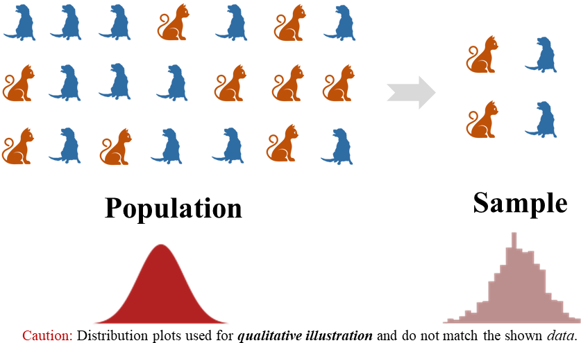
• Underlying unknown distribution (left)
• Empirical distribution of the available sample (right)

from scipy import stats # https://docs.scipy.org/doc/scipy/reference/tutorial/stats.html
np.random.seed(seed=5)
x = np.linspace(-3, 3, 300) # Return evenly spaced numbers over the specified interval
xsample = stats.norm.rvs(size=1000) # generate 1000 random variates for 'norm'al distribution
fig, axes = plt.subplots(ncols=2, figsize=(6, 2.7))
ax = axes[0]
ax.fill(x, stats.norm.pdf(x),'firebrick') # Probability Density Function
ax.set_axis_off()
ax.set_xlim(-3, 3)
ax = axes[1]
ax.hist(xsample, bins=100,color='rosybrown') # Histogram of the random variate samples
ax.set_axis_off()
ax.set_xlim(-3, 3)
ax.set_position
# plt.subplots_adjust(left=0, bottom=0, right=1, top=1, wspace=0, hspace=0)
plt.show()

Big data & sampling

• Now that we have scalable Big data processing tools, why bother with samples?

• quality of the data collection may vary
  • e.g., in an IoT set-up, sensors may have different degrees of defectiveness

• the data may not be representative
  • e.g., using social media data to gauge the nation's sentiment
    • are all sections of the society rightly represented on social media?

• time and effort spent on random sampling may help reduces bias and make it easier to explore
  • visualize and manually interpret information (including missing data/outliers)

(Uniform) random sampling

• each available member of the population being sampled has an equal chance of being chosen
  • with replacement: observations are put back in the population after each draw
    • for possible future reselection
  • without replacement
    • once selected, unavailable for future draws

• Stratified sampling: Dividing the population into strata and randomly sampling from each strata.
• Without stratification
  • a.k.a. simple random sampling

2020 US presidential election	FiveThirtyEight projection

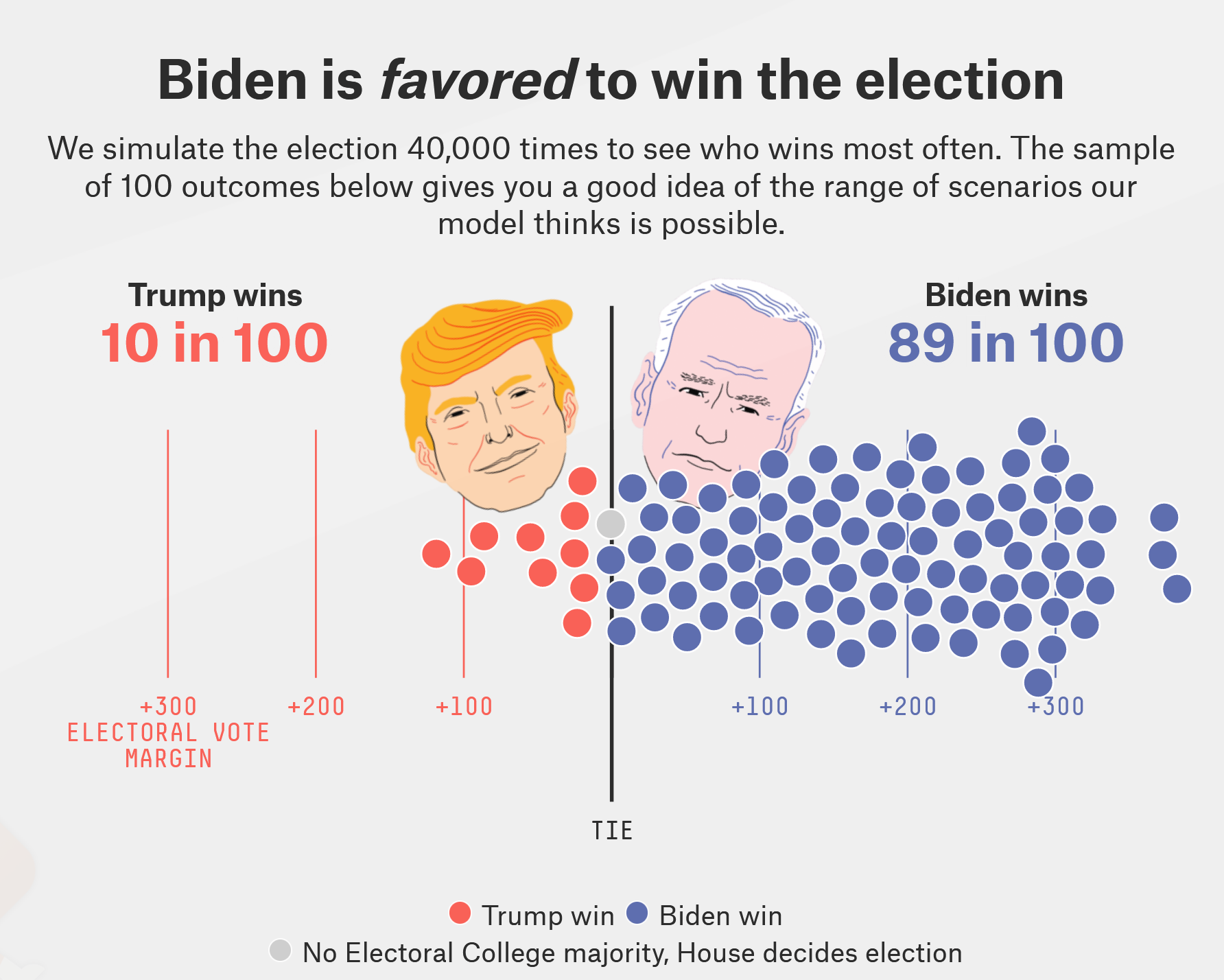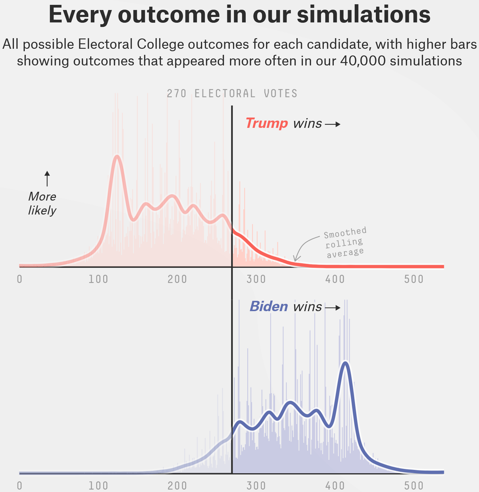Screenshots from https://projects.fivethirtyeight.com/2020-election-forecast/

Bias

• Not always obvious how to get a good random sample
  • e.g., customer behavior: time of the day, day of the week, period of the year
  • Anecdotes: The literary digest presidential poll of 1936
    • Polled ten million individuals, of whom 2.27 million responded
    • The magnitude of the magazine's error: 39.08% for the popular vote for Roosevelt v Landon
    • Gallup correctly predicted the results using a much smaller sample size of just 50,000
    • Contemporary claim to fame Nate Silver & FiveThirtyEight
      • "balance out the polls with comparative demographic data"

• Selection bias: selectively choosing data—consciously or unconsciously—in a way that leads to a conclusion that is misleading or ephemeral
  • e.g., Regression to the mean: Is your coin really 'lucky'?

• Data snooping: extensive hunting through data in search of something interesting
  • e.g., Crowd-sourced coin tossing to find a `lucky coin'
• Vast search effect: Bias or nonreproducibility resulting from repeated data modeling, or modeling data with large numbers of predictor variables.
  • Beware the promise of Big Data: You can run many models and ask many questions. But is it really a needly that you find in the haystack?
    • Mitigations: Holdout set, Target shuffling

Methodology check-point

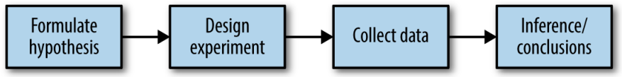
• Specify hypothesis first, then design experiment and accordingly collect data following randomization principles to avoid falling into the traps of biases
• Traps of biases resulting from the data collection/analysis process:
  • repeated running of models in data mining & data snooping
  • after-the-fact selection of interesting events

Sampling distribution of a statistic

Sampling distribution: distribution of some sample statistic over many samples drawn from the same population.

Standard error: The variability (standard deviation) of a sample statistic over many samples (not to be confused with standard deviation, which by itself, refers to variability of individual data values)

Central Limit Theorem: The tendency of the sampling distribution to take on a normal shape as the sample size rises.

g = sns.FacetGrid(results, col='type', col_wrap=4, height=3, aspect=1)
g.map(plt.hist, 'income', range=[0, 200000], bins=40, facecolor='gainsboro')
g.set_axis_labels('Income', 'Count')
g.set_titles('{col_name}')
g.fig.suptitle('Visualizing Central Limit Theorem in action')
plt.tight_layout()
plt.show()

Confidence interval

• x% confidence interval: It is the interval that encloses the central x% of the bootstrap sampling distribution of a sample statistic
• Bootstrap sampling based confidence interval computation
  1. Draw a random sample of size n with replacement from the data (a resample)
  2. Record the statistic of interest for the resample
  3. Repeat steps 1–2 many (R) times
  4. For an x% confidence interval, trim [(100-x) / 2]% of the R resample results from either end of the distribution
  5. The trim points are the endpoints of an x% bootstrap confidence interval

from sklearn.utils import resample
#print('Data Mean: '+str(loans_income.mean()))
np.random.seed(seed=3)  
# create a sample of 20 loan income data
#sample20 = resample(loans_income, n_samples=20, replace=False)
#print('Sample Mean: '+str(sample20.mean()))
results = []
for _ in range(500):
    sample = resample(loans_income, n_samples=20, replace=True)
    #sample = resample(sample20) # One could also use a small initial sample, to keep re-sampling
    results.append(sample.mean())
results = pd.Series(results)

confidence_interval = list(results.quantile([0.05, 0.95]))

ax = results.plot.hist(bins=30, facecolor='gainsboro', figsize=(4.5,3.5))
ax.plot(confidence_interval, [55, 55], color='black')
for x in confidence_interval:
    ax.plot([x, x], [0, 65], color='black')
    ax.text(x, 70, f'{x:.0f}', horizontalalignment='center', verticalalignment='center')
ax.text(sum(confidence_interval) / 2, 60, '90% interval', horizontalalignment='center', verticalalignment='center')
meanIncome = results.mean()
ax.plot([meanIncome, meanIncome], [0, 50], color='black', linestyle='--')
ax.text(meanIncome, 10, f'Mean: {meanIncome:.0f}', bbox=dict(facecolor='white', edgecolor='white', alpha=0.5),
        horizontalalignment='center', verticalalignment='center')
ax.set_ylim(0, 80)
ax.set_ylabel('Counts')
plt.tight_layout()
plt.show()

Interpreting confidence interval

A note of caution: Confidence interval DOES NOT answer the question “What is the probability that the true value lies within a certain interval?”

Statistical experiments & significance

In 2012 a Microsoft employee working on Bing had an idea about changing the way the search engine displayed ad headlines. Developing it wouldn’t require much effort—just a few days of an engineer’s time—but it was one of hundreds of ideas proposed, and the program managers deemed it a low priority. So it languished for more than six months, until an engineer, who saw that the cost of writing the code for it would be small, launched a simple online controlled experiment—an A/B test—to assess its impact. Within hours the new headline variation was producing abnormally high revenue, triggering a “too good to be true” alert. Usually, such alerts signal a bug, but not in this case. An analysis showed that the change had increased revenue by an astonishing 12%—which on an annual basis would come to more than $100 million in the United States alone—without hurting key user-experience metrics. It was the best revenue-generating idea in Bing’s history, but until the test its value was underappreciated.

Source: https://hbr.org/2017/09/the-surprising-power-of-online-experiments

Statistical inference pipeline

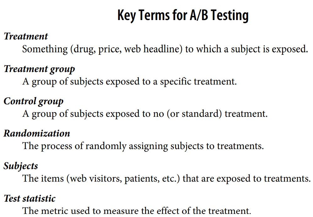
Design experiment (typically, an A/B test): An A/B test is an experiment with two groups to establish which of two treatments, products, procedures, or the like is superior. Often one of the two treatments is the standard existing treatment, or no treatment. If a standard (or no) treatment is used, it is called the control. A typical hypothesis is that a new treatment is better than the control.

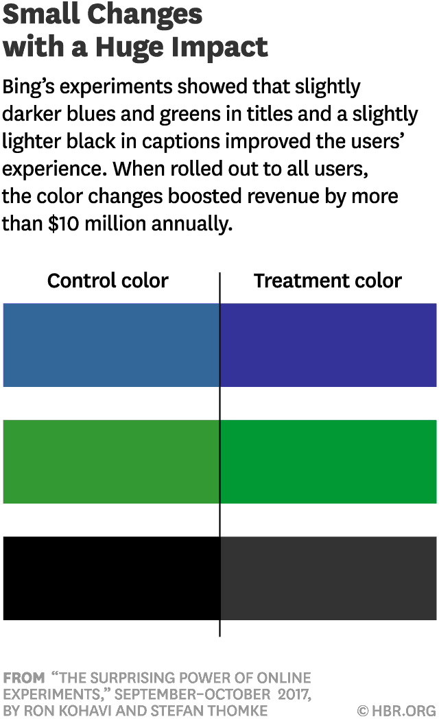
Image source: Harvard Business Review

Randomization

• Ideally, subjects ought to be assigned randomly to treatments.
• Then, any difference between the treatment groups is due to one of two things
  • Effect of different treatments
  • Luck of the draw
    • Ideal randomization may not always be possible

Control group

• Why not just compare with the original baseline?
  • Without a control group, there is no assurance that “all other things are equal”

Blinding

• Blind study: A blind study is one in which the subjects are unaware of whether they are getting treatment A or treatment B
• Double-blind study: A double-blind study is one in which the investigators and facilitators also are unaware which subjects are getting which treatment
  • Blinding maynot always be feasible

Ethical & legal considerations

• In the context of web applications and data products, do you need permission to carry out the study?
  • Anecdotes
    • Facebook's emotion study on its feeds was hugely controversial
    • OKCupid's study on compatibilty & matches

Interpreting A/B test results with statistical rigour

• Human brain/intuition is (typically) not good at comprehending or interpreting randomness
• Hypothesis testing

  Assess whether random chance is a reasonable explanation for the observed difference between treatment groups

Hypothesis testing

• Null hypothesis $H_{0}$
• Alternative hypothesis $H_1$
  • Variations:
    • one-way/one-tail, e.g. $H_{0} \leq \mu $, $H_1 > \mu$
    • two-way/two-tail, e.g., $H_{0} = \mu$, $H_1 \neq \mu$
• Caution: One only rejects, or fails to reject the Null hypothesis
  • DOES NOT PROVE anything
    • May nevertheless be `good enough' for a lot of decisions

Resampling

Resampling in statistics means to repeatedly sample values from observed data, with a general goal of assessing random variability in a statistic

Broadly, two variations:

• Bootstrap
  • We saw this variant earlier, when exposing the idea of Central Limit Theorem
• Permutation tests
  • Typically, this is what is used for hypothesis testing
    • A special case is an exhaustive permutation test (practical only for small data sets)

Permutation test

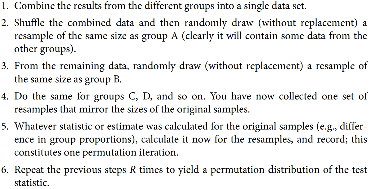
Permutation test

Compare observed difference between groups and to the set of permuted differences.

If the observed difference lies well within the set of permuted differences

• Can NOT reject Null hypothesis

Else

• The difference is statistically significant, i.e., reject Null hypothesis

Web stickiness example

# Data
session_times = pd.read_csv(practicalstatspath+'web_page_data.csv')
session_times.Time = 100 * session_times.Time
session_times.head()

	Page	Time
0	Page A	21.0
1	Page B	253.0
2	Page A	35.0
3	Page B	71.0
4	Page A	67.0

# Understanding the data visually
ax = session_times.boxplot(by='Page', column='Time', figsize=(4, 4))
ax.set_xlabel('')
ax.set_ylabel('Time (in seconds)')
plt.suptitle('')

plt.tight_layout()
plt.show()

# We will use "mean" as the statistics
mean_a = session_times[session_times.Page == 'Page A'].Time.mean()
mean_b = session_times[session_times.Page == 'Page B'].Time.mean()
print(mean_b - mean_a)

35.66666666666667

# Permutation test example with stickiness
# Creating the permutation functionality
def perm_fun(x, nA, nB):
    n = nA + nB
    idx_B = set(random.sample(range(n), nB))
    idx_A = set(range(n)) - idx_B
    return x.loc[idx_B].mean() - x.loc[idx_A].mean()
    
nA = session_times[session_times.Page == 'Page A'].shape[0]
nB = session_times[session_times.Page == 'Page B'].shape[0]
print(perm_fun(session_times.Time, nA, nB))

-8.790476190476198

# Repeating the permutation experiment R times
R=1000
random.seed(1) # Using a seed helps make the randomized expeirments deterministic
perm_diffs = [perm_fun(session_times.Time, nA, nB) for _ in range(R)]

fig, ax = plt.subplots(figsize=(5, 3.54))
ax.hist(perm_diffs, bins=21, rwidth=0.9,facecolor='gainsboro')
ax.axvline(x = mean_b - mean_a, color='black', lw=1)
ax.text(40, 100, 'Observed\ndifference')
ax.set_xlabel('Session time differences (in seconds)')
ax.set_ylabel('Frequency')

plt.tight_layout()
plt.show()

p-value

In what fraction of permutations does the difference in means exceed the observed difference?

len([x for x in perm_diffs if x > (mean_b - mean_a)])/len(perm_diffs)

0.121

In what fraction of permutations does the difference in means exceed the observed difference?

A rather large fraction!

For the observed difference to be "meaningful", it needs to be outside the range of chance variation. Otherwise, it is NOT statistically significant.

Therefore, we do NOT reject the Null hypothesis

Smaller the p-value, stronger the evidence to reject the Null hypothesis

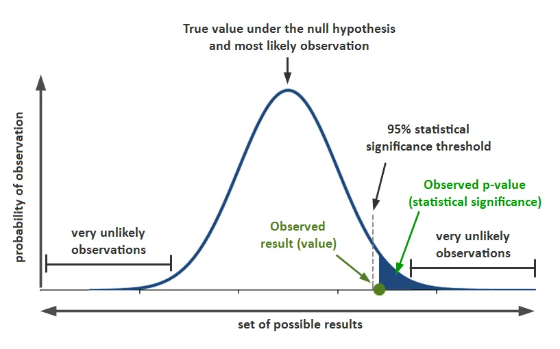
Image source: https://www.simplypsychology.org/p-value.html

Level of confidence, singnificance & p-value

• Choose the rigour of your statistical test upfront:
  • Level of confidence: $C$
  • Level of significance $\alpha=1-C$

    If p-value is smaller than $\alpha$ then reject Null hypothesis!

What p-value represents:

The probability that, given a chance model, results as extreme as the observed results could occur.

What p-value does NOT represent:

The probability that the result is due to chance. (which is what, one would ideally like to know!)

Errors

Type-1 error: Mistakenly conclude an effect is real (and thus, reject the Null hypothesis), when it is really just due to chance

• Related to the concept of precision (more nuances apply)

Type-2 error: Mistakenly conclude that an effect is not real, i.e., due to chance (and thus fail to reject the Null hypothesis), when it actually is real

• In the context of hypothesis testing, generally an issue of inadequate data
• Complement of recall

ANOVA: Analysis of Variance

Web stickiness example with 4 pages

four_sessions = pd.read_csv(practicalstatspath+'four_sessions.csv')

ax = four_sessions.boxplot(by='Page', column='Time', figsize=(4, 4))
ax.set_xlabel('Page')
ax.set_ylabel('Time (in seconds)')
plt.suptitle('')
plt.title('')

plt.tight_layout()
plt.show()

Could all the pages have the same underlying stickiness, and the differences among them be due to randomness?

• Null hypothesis: Pages do not have under distinct stickiness
• Alternative hypothesis: Pages do have statistically significant distinct stickiness
  • Target level of confidence: 95%

print('Observed means:', four_sessions.groupby('Page').mean().values.ravel())
observed_variance = four_sessions.groupby('Page').mean().var()[0]
print('Variance:', observed_variance)
# Permutation test example with stickiness
# Usually you will permute a small subset of each kind, but in this example, the data is small as is
def perm_test(df):
    df = df.copy()
    df['Time'] = np.random.permutation(df['Time'].values)
    return df.groupby('Page').mean().var()[0]
    
print(perm_test(four_sessions))

Observed means: [172.8 182.6 175.6 164.6]
Variance: 55.426666666666655
18.94666666666669

random.seed(1)
perm_variance = [perm_test(four_sessions) for _ in range(1000)]
p_val=np.mean([var > observed_variance for var in perm_variance])
print('p-value: ', p_val)
if p_val<0.05:
    print('Null hypothesis rejected')
else:
    print('Null hypothesis CANNOT be rejected')

p-value:  0.083
Null hypothesis CANNOT be rejected

fig, ax = plt.subplots(figsize=(5, 3.54))
ax.hist(perm_variance, bins=11, rwidth=0.9,facecolor='gainsboro')
ax.axvline(x = observed_variance, color='black', lw=1)
ax.text(58, 180, 'Observed\nvariance')
ax.set_xlabel('Variance')
ax.set_ylabel('Frequency')

plt.tight_layout()
plt.show()

Pragmatic (data product) practioner and statistical tests!

Conduct A/A tests

Be careful about assumptions of causality

• Anecdotes
  • Microsoft Office's advanced features/attrition experiment
    • Two teams conducted separate observational studies of two advanced features for Microsoft Office. Each concluded that the new feature it was assessing reduced attrition.
  • Yahoo's experiment on whether the display of ads for a brand increase searches for the brand name or related keywords
    • Importance of control.

Complex experiment designs and chance of bugs in experiment design/data collection

Sometime's understanding the "why?" is useful, but sometimes, you may have to just go with whatever "floats your boat"!

• Scurvy versus Bing's design color

Suggested additional readings and references

Data-Driven Metric Development for Online Controlled Experiments: Seven Lessons Learned by Deng & Shi at KDD 2016

The Surprising Power of Online Experiments by Ron Kohavi and Stefan Thomke, Harvard Business Review

A compilation of numerous statistical tests with Python code snippets (Good collection of Python statistical test APIs. However, the content has not been vetted for correctness by me. Apply your own caution, particularly regarding the suggested interpretation of the tests.)