Data Privacy Enhancing Techniques
SC 4125: Developing Data Products
Module-8: Data Governance/Privacy Issues
by Anwitaman DATTA
School of Computer Science and Engineering, NTU Singapore.
Disclaimer/Caveat emptor
- Non-systematic and non-exhaustive review
- Illustrative approaches are not necessarily the most efficient or elegant, let alone unique
- This Jupyter notebook is accompanied by a deck of slides discussing Data Governance in general, as well as specific privacy enhancing techniques.
Acknowledgement
This module is adapted from workshop training material created by Andreas Dewes and Katherine Jarmul from Kiprotect, which they have made available under MIT License. Here's an accompanying talk on Data Science Meets Data Protection.
If anyone reuses the material in the current format as readapted and provided here, please still also attribute the original creators of the content.
If there are any attribution omissions to be rectified, or should anything in the material need to be changed or redacted, the copyright owners are requested to contact me at anwitaman@ntu.edu.sg
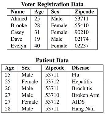
k-Anonymity
| External data (voter registration information) can be used to deanonymyze | 2-Anonymyzed patient data |
|---|---|
 |
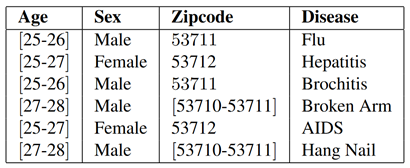 |
Example from Mondrian Multidimensional K-Anonymity by LeFevre et al
# this is a list of the column names in our dataset (the file doesn't contain headers)
names = (
    'age',
    'workclass', #Private, Self-emp-not-inc, Self-emp-inc, Federal-gov, Local-gov, State-gov, Without-pay, Never-worked.
    'fnlwgt', # final weight. In other words, this is the number of people the census believes the entry represents.
    'education',
    'education-num',
    'marital-status',
    'occupation',
    'relationship',
    'race',
    'sex',
    'capital-gain',
    'capital-loss',
    'hours-per-week',
    'native-country',
    'income',
)
# some fields are categorical and thus they need to be treated accordingly
# note that integers are used to represent some of the categorical data
categorical = set((
    'workclass',
    'education',
    'marital-status',
    'occupation',
    'relationship',
    'sex',
    'native-country',
    'race',
    'income',
))
import pandas as pd
datapath ='data/kiprotectdata/' # change this to adjust relative path
df = pd.read_csv(datapath+"adult.all.txt", sep=", ", header=None, names=names, index_col=False, engine='python')
for name in categorical:
    df[name] = df[name].astype('category')
print(df.shape)
df.sample(10)
(48842, 15)
| age | workclass | fnlwgt | education | education-num | marital-status | occupation | relationship | race | sex | capital-gain | capital-loss | hours-per-week | native-country | income | |
|---|---|---|---|---|---|---|---|---|---|---|---|---|---|---|---|
| 38515 | 37 | Private | 285637 | HS-grad | 9 | Never-married | Transport-moving | Not-in-family | Black | Male | 0 | 0 | 50 | United-States | <=50k |
| 19744 | 57 | Private | 29375 | HS-grad | 9 | Separated | Sales | Not-in-family | Amer-Indian-Eskimo | Female | 0 | 0 | 35 | United-States | <=50k |
| 9584 | 19 | Private | 201743 | Some-college | 10 | Never-married | Other-service | Own-child | White | Female | 0 | 0 | 26 | United-States | <=50k |
| 18273 | 23 | State-gov | 35633 | Some-college | 10 | Never-married | Other-service | Not-in-family | White | Male | 0 | 0 | 50 | United-States | <=50k |
| 14838 | 32 | Self-emp-inc | 161153 | HS-grad | 9 | Married-civ-spouse | Farming-fishing | Husband | White | Male | 0 | 1902 | 55 | United-States | >50k |
| 16585 | 44 | Private | 192381 | Bachelors | 13 | Married-civ-spouse | Prof-specialty | Husband | White | Male | 0 | 1848 | 40 | United-States | >50k |
| 22570 | 43 | Self-emp-inc | 602513 | Masters | 14 | Married-civ-spouse | Exec-managerial | Husband | White | Male | 0 | 0 | 50 | United-States | >50k |
| 25297 | 69 | Federal-gov | 143849 | 11th | 7 | Widowed | Adm-clerical | Not-in-family | White | Female | 0 | 0 | 20 | United-States | <=50k |
| 39942 | 35 | Private | 351772 | Some-college | 10 | Married-civ-spouse | Sales | Husband | White | Male | 0 | 0 | 60 | United-States | >50k |
| 4431 | 21 | Private | 174503 | HS-grad | 9 | Never-married | Adm-clerical | Not-in-family | White | Female | 0 | 0 | 30 | United-States | <=50k |
Greedy heuristic
Helper function: spans of columns of a dataframe
We first need a function that returns the spans (max-min for numerical columns, number of different values for categorical columns) of all columns for a partition of a dataframe.
def get_spans(df, partition, scale=None):
    """
    :param        df: the dataframe for which to calculate the spans
    :param partition: the partition for which to calculate the spans
    :param     scale: if given, the spans of each column will be divided
                      by the value in `scale` for that column
    :        returns: The spans of all columns in the partition
    """
    spans = {}
    for column in df.columns:
        if column in categorical:
            span = len(df[column][partition].unique())
        else:
            span = df[column][partition].max()-df[column][partition].min()
        if scale is not None:
            span = span/scale[column]
        spans[column] = span
    return spans
full_spans = get_spans(df, df.index)
full_spans
{'age': 73,
 'workclass': 9,
 'fnlwgt': 1478115,
 'education': 16,
 'education-num': 15,
 'marital-status': 7,
 'occupation': 15,
 'relationship': 6,
 'race': 5,
 'sex': 2,
 'capital-gain': 99999,
 'capital-loss': 4356,
 'hours-per-week': 98,
 'native-country': 42,
 'income': 2}
Helper function: split a dataframe in two partitions based on a column
partition the dataframe, returning two partitions such that
- all rows with values of a chosen/indicated column
columnbelow the median are in one partition- all rows with values above or equal to the median are in the other
- for categorical data, divide them into two disjoint sets of (roughly) equal number of categories
def split(df, partition, column):
    """
    :param        df: The dataframe to split
    :param partition: The partition to split
    :param    column: The column along which to split
    :        returns: A tuple containing a split of the original partition
    """
    dfp = df[column][partition]
    if column in categorical:
        values = dfp.unique()
        lv = set(values[:len(values)//2])
        rv = set(values[len(values)//2:])
        return dfp.index[dfp.isin(lv)], dfp.index[dfp.isin(rv)]
    else:
        median = dfp.median()
        dfl = dfp.index[dfp < median]
        dfr = dfp.index[dfp >= median]
        return (dfl, dfr)
Helper function: Determines if a specific partition has at least k entrees
def is_k_anonymous(df, partition, sensitive_column, k=5):
    """
    :param               df: The dataframe on which to check the partition.
    :param        partition: The partition of the dataframe to check.
    :param sensitive_column: The name of the sensitive column
    :param                k: The desired k
    :returns               : True if the partition is valid according to our k-anonymity criteria, False otherwise.
    """
    if len(partition) < k:
        return False
    return True
Greedy partitioning
def partition_dataset(df, feature_columns, sensitive_column, scale, is_valid):
    """
    :param               df: The dataframe to be partitioned.
    :param  feature_columns: A list of column names along which to partition the dataset.
    :param sensitive_column: The name of the sensitive column (to be passed on to the `is_valid` function)
    :param            scale: The column spans as generated before.
    :param         is_valid: A function that takes a dataframe and a partition and returns True if the partition is valid.
    :returns               : A list of valid partitions that cover the entire dataframe.
    """
    finished_partitions = []
    partitions = [df.index]
    while partitions:
        partition = partitions.pop(0)
        spans = get_spans(df[feature_columns], partition, scale)
        for column, span in sorted(spans.items(), key=lambda x:-x[1]):
            #we try to split this partition along a given column
            lp, rp = split(df, partition, column)
            if not is_valid(df, lp, sensitive_column) or not is_valid(df, rp, sensitive_column):
                continue
            # the split is valid, we put the new partitions on the list and continue
            partitions.extend((lp, rp))
            break
        else:
            # no split was possible, we add the partition to the finished partitions
            finished_partitions.append(partition)
    return finished_partitions
# we apply the partitioning method to two columns of the dataset, using "income" as the sensitive attribute
feature_columns = ['age', 'education-num']
sensitive_column = 'income'
finished_partitions = partition_dataset(df, feature_columns, sensitive_column, full_spans, is_k_anonymous)
print(len(finished_partitions))
460
Visualizing the partitioning achieved
import matplotlib.pyplot as plt
import matplotlib.patches as patches
part_sizes=[len(x) for x in finished_partitions]
plt.hist(part_sizes,bins=200,log=True)
plt.ylabel('# of partitions (log)')
plt.xlabel('size of partition');

# Details of plotting function plot_rects has been skipped in the slide: Check the Jupyter notebook
plt.figure(figsize=(15,8))
ax = plt.subplot()
plot_rects(df, ax, rects, column_x, column_y, facecolor='r')
# we can also plot the datapoints themselves
plt.scatter(df[column_x], df[column_y])
<matplotlib.collections.PathCollection at 0x1cd73578340>

Generating the k-anonymous dataset
So far we have identified the partition boundaries, along which to group the data items.
- We need to aggregate data within the partitions, to create the k-anonymous dataset.
def agg_categorical_column(series):
    return [','.join(set(series))]

def agg_numerical_column(series):
    return [series.mean()]
# Caution: I have tested it with other feature_columns choices and the code is brittle and it breaks.
# It serves the pedagogical purpose, but you may have to fix/reimplement for general purpose use.
def build_anonymized_dataset(df, partitions, feature_columns, sensitive_column, max_partitions=None):
    aggregations = {}
    for column in feature_columns:
        if column in categorical:
            aggregations[column] = agg_categorical_column
        else:
            aggregations[column] = agg_numerical_column
    rows = []
    for i, partition in enumerate(partitions):
        #if i % 100 == 1:
        #    print("Finished {} partitions...".format(i))
        if max_partitions is not None and i > max_partitions:
            break
        grouped_columns = df.loc[partition].agg(aggregations, squeeze=False)
        sensitive_counts = df.loc[partition].groupby(sensitive_column).agg({sensitive_column : 'count'})
        values = grouped_columns.iloc[0].to_dict()
        for sensitive_value, count in sensitive_counts[sensitive_column].items():
            if count == 0:
                continue
            values.update({
                sensitive_column : sensitive_value,
                'count' : count,
            })
            rows.append(values.copy())

    return pd.DataFrame(rows)
# we sort the resulting dataframe using the feature columns and the sensitive attribute
dfn=build_anonymized_dataset(df, finished_partitions, feature_columns, sensitive_column)\
      .sort_values(feature_columns+[sensitive_column])
dfn
| age | education-num | income | count | |
|---|---|---|---|---|
| 605 | 17.0 | 4.000000 | <=50k | 5 |
| 110 | 17.0 | 5.000000 | <=50k | 36 |
| 111 | 17.0 | 6.000000 | <=50k | 198 |
| 0 | 17.0 | 7.200599 | <=50k | 334 |
| 120 | 17.0 | 9.000000 | <=50k | 14 |
| ... | ... | ... | ... | ... |
| 726 | 90.0 | 9.000000 | >50k | 4 |
| 736 | 90.0 | 10.545455 | <=50k | 9 |
| 737 | 90.0 | 10.545455 | >50k | 2 |
| 772 | 90.0 | 14.000000 | <=50k | 2 |
| 773 | 90.0 | 14.000000 | >50k | 3 |
776 rows × 4 columns
Ungraded task
Ungraded Task 8.1.i: Generate k-anonymous, l-diverse dataset.
Hint: You need minor modification to how/when partitioning is done.
Ungraded Task 8.1.ii: For a dataset of your choice, train a ML model (of your choice) with the raw data versus the k-anonymyzed data and compare their performances (you may use default parameter choices, or try to optimize for each case).
Note: When using k-anonymyzed data to train, the test data could still be the way the original "raw" data was.
Ungraded Task 8.2: Generate differentially private data from the census dataset, using the same set of features and sensitive columns. Benchmark the performance of models trained with different parameter choices, comparing with the model built using the original (non-noisy) data.
Hint: There are only two categories for the sensitive (income) data.