A little bit of SQL(ite)

and very little Pandas

SC 4125: Developing Data Products

Module-1: Introduction

by Anwitaman DATTA
School of Computer Science and Engineering, NTU Singapore.

Teaching material

• .pdf deck of slides (complements the html slides)
• .html deck of slides
• .ipynb Jupyter notebook

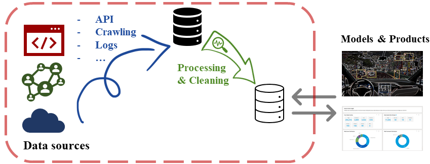
This is companion material for Module-1: Introduction lecture for the Developing Data Products course.

The executable source .ipynb notebook file for these HTML slides, and the CountriesDB.db file that goes with it can be found through the links.

A very non-systematic review/recap

You are expected to have already taken introductory courses

• SC 1015: Introduction to Data Science & AI
• SC 2207: Introduction to Database Systems

Some useful references for beginners/catching-up:

https://www.sqlitetutorial.net/

https://pandas.pydata.org/pandas-docs/stable/getting_started/tutorials.html

SQLite Browser

https://sqlitebrowser.org/

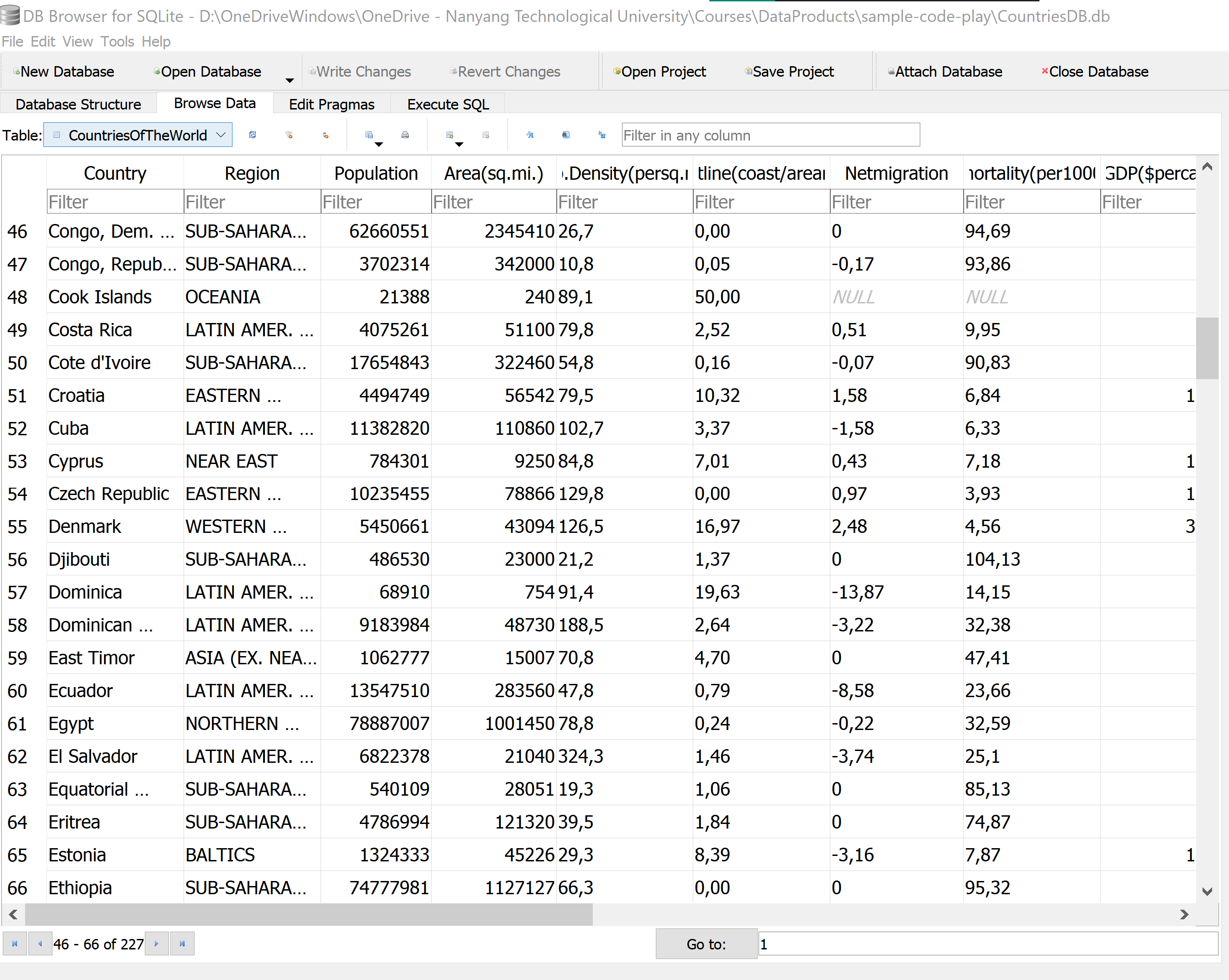
This notebook is accompanied with CountriesDB.db file, which comprises of three tables. The tables correspond to the Countries of the world and gapminder data obtained from Kaggle, and the Olympics 2016 medals data obtained from Wikipedia.

You may want to install and use the SQLite Browser to check out the data in the .db file (as shown in the previous panel). You may also want to check out the source files indicated above.

It is easy to import the .csv (and other similar formats, such as .tsv) directly using the graphical interface of SQLite Browser. Nevertheless, we will next explore how to do so, and other actions such as manipulate and query the data from the Jupyter programming environment.

Import modules

Let's start with importing necessary modules. We will also check the environment/version/etc.

# Housekeeping: We will first carry out the imports and print version numbers
import sys
print("Python version: " +str(sys.version))
import numpy as np
import pandas as pd
print("Numpy version: " +str(np.version.version))
print("Pandas version: " +str(pd.__version__))

#import xml.etree.ElementTree as ET
import sqlite3
print("SQLite version: " + str(sqlite3.version))

Python version: 3.8.5 (default, Sep  3 2020, 21:29:08) [MSC v.1916 64 bit (AMD64)]
Numpy version: 1.19.2
Pandas version: 1.1.3
SQLite version: 2.6.0

! jupyter --version

jupyter core     : 4.6.3
jupyter-notebook : 6.1.4
qtconsole        : 4.7.7
ipython          : 7.19.0
ipykernel        : 5.3.4
jupyter client   : 6.1.7
jupyter lab      : 3.0.16
nbconvert        : 6.0.7
ipywidgets       : 7.5.1
nbformat         : 5.0.8
traitlets        : 5.0.5

We begin by connecting to the CountriesDB.db database, using the sqlite3.connect() function.

conn = sqlite3.connect('CountriesDB.db')

We then create a cursor object using the cursor() function. We determine the tables stored in the database, we can query (using a SELECT statement) a special table called the sqlite_schema. It can also be referenced as sqlite_master.

To retrieve data after executing a SELECT statement, one can either treat the cursor as an iterator, call the cursor’s fetchone() method to retrieve a single matching row, or call fetchall() to get a list of the matching rows.

cursor = conn.cursor()
cursor.execute("SELECT name FROM sqlite_schema WHERE type='table';")
db_tables= [x[0] for x in cursor.fetchall()] # we are storing this information in a list
print(db_tables)

['CountriesOfTheWorld', 'gapminder', 'Olymp2016']

If we want to determine the schema of one of these tables, say, the gapminder table, we may achieve it as follows.

cursor.execute("SELECT sql FROM sqlite_master WHERE name = 'gapminder';")
print(cursor.fetchall())

[('CREATE TABLE "gapminder" (\n\t"country"\tTEXT,\n\t"continent"\tTEXT,\n\t"year"\tINTEGER,\n\t"lifeExp"\tREAL,\n\t"pop"\tINTEGER,\n\t"gdpPercap"\tREAL\n)',)]

Alternatively, we may also use the description method to determine the schema instead.

data=cursor.execute("SELECT * FROM 'gapminder'")
data_descr=[x[0] for x in data.description]
print(data_descr)

['country', 'continent', 'year', 'lifeExp', 'pop', 'gdpPercap']

# If you do not want to type the names, you can ofcourse 
# refer to the db_tables and iterate as needed.
data=cursor.execute('SELECT * FROM ' +str(db_tables[0]))
data_descr=[x[0] for x in data.description]
print(data_descr)

['Country', 'Region', 'Population', 'Area(sq.mi.)', 'Pop.Density(persq.mi.)', 'Coastline(coast/arearatio)', 'Netmigration', 'Infantmortality(per1000births)', 'GDP($percapita)', 'Literacy(%)', 'Phones(per1000)', 'Arable(%)', 'Crops(%)', 'Other(%)', 'Climate', 'Birthrate', 'Deathrate', 'Agriculture', 'Industry', 'Service']

How do we check the data itself? Depending on the purpose, we can obtain it in different manners. We have already seen the most basic option, of carrying out a cursor.execute() followed by fetchone()/fetchall().

One can also instead just carry out a pandas read_sql_query, and store the result in a dataframe.

Countries_df = pd.read_sql_query("SELECT * FROM CountriesOfTheWorld", conn) # we need to provide the DB connection information
Countries_df

	Country	Region	Population	Area(sq.mi.)	Pop.Density(persq.mi.)	Coastline(coast/arearatio)	Netmigration	Infantmortality(per1000births)	GDP($percapita)	Literacy(%)	Phones(per1000)	Arable(%)	Crops(%)	Other(%)	Climate	Birthrate	Deathrate	Agriculture	Industry	Service
0	Afghanistan	ASIA (EX. NEAR EAST)	31056997	647500	48,0	0,00	23,06	163,07	700.0	36,0	3,2	12,13	0,22	87,65	1	46,6	20,34	0,38	0,24	0,38
1	Albania	EASTERN EUROPE	3581655	28748	124,6	1,26	-4,93	21,52	4500.0	86,5	71,2	21,09	4,42	74,49	3	15,11	5,22	0,232	0,188	0,579
2	Algeria	NORTHERN AFRICA	32930091	2381740	13,8	0,04	-0,39	31	6000.0	70,0	78,1	3,22	0,25	96,53	1	17,14	4,61	0,101	0,6	0,298
3	American Samoa	OCEANIA	57794	199	290,4	58,29	-20,71	9,27	8000.0	97,0	259,5	10	15	75	2	22,46	3,27	None	None	None
4	Andorra	WESTERN EUROPE	71201	468	152,1	0,00	6,6	4,05	19000.0	100,0	497,2	2,22	0	97,78	3	8,71	6,25	None	None	None
...	...	...	...	...	...	...	...	...	...	...	...	...	...	...	...	...	...	...	...	...
222	West Bank	NEAR EAST	2460492	5860	419,9	0,00	2,98	19,62	800.0	None	145,2	16,9	18,97	64,13	3	31,67	3,92	0,09	0,28	0,63
223	Western Sahara	NORTHERN AFRICA	273008	266000	1,0	0,42	None	None	NaN	None	None	0,02	0	99,98	1	None	None	None	None	0,4
224	Yemen	NEAR EAST	21456188	527970	40,6	0,36	0	61,5	800.0	50,2	37,2	2,78	0,24	96,98	1	42,89	8,3	0,135	0,472	0,393
225	Zambia	SUB-SAHARAN AFRICA	11502010	752614	15,3	0,00	0	88,29	800.0	80,6	8,2	7,08	0,03	92,9	2	41	19,93	0,22	0,29	0,489
226	Zimbabwe	SUB-SAHARAN AFRICA	12236805	390580	31,3	0,00	0	67,69	1900.0	90,7	26,8	8,32	0,34	91,34	2	28,01	21,84	0,179	0,243	0,579

227 rows × 20 columns

We will next create the Olymp2016 table using data from Wikipedia for the Rio 2016 Olympics.

Let's start by reading the data from the Wikipedia page. The read_html() method works neatly (assuming that the HTML source file itself is constructed neatly, otherwise, it may get miserable!). The read_html() obtains several tables. After inspection of the results, it turned out that the table indexed '2' is the medal tally table for the specific Wiki-page (as on 9th August 2021).

olymp_df=pd.read_html(r'https://en.wikipedia.org/wiki/2016_Summer_Olympics_medal_table')
olymp2016medals=olymp_df[2]
olymp2016medals

	Rank	NOC	Gold	Silver	Bronze	Total
0	1	United States (USA)	46	37	38	121
1	2	Great Britain (GBR)	27	23	17	67
2	3	China (CHN)	26	18	26	70
3	4	Russia (RUS)	19	17	20	56
4	5	Germany (GER)	17	10	15	42
...	...	...	...	...	...	...
82	78	Nigeria (NGR)	0	0	1	1
83	78	Portugal (POR)	0	0	1	1
84	78	Trinidad and Tobago (TTO)	0	0	1	1
85	78	United Arab Emirates (UAE)	0	0	1	1
86	Totals (86 NOCs)	Totals (86 NOCs)	307	307	359	973

87 rows × 6 columns

We do not want to populate the database with a derived information of Totals, and wish to eliminate the last line. Let's try that!

olymp2016medals=olymp_df[2][:-1]
olymp2016medals

	Rank	NOC	Gold	Silver	Bronze	Total
0	1	United States (USA)	46	37	38	121
1	2	Great Britain (GBR)	27	23	17	67
2	3	China (CHN)	26	18	26	70
3	4	Russia (RUS)	19	17	20	56
4	5	Germany (GER)	17	10	15	42
...	...	...	...	...	...	...
81	78	Morocco (MAR)	0	0	1	1
82	78	Nigeria (NGR)	0	0	1	1
83	78	Portugal (POR)	0	0	1	1
84	78	Trinidad and Tobago (TTO)	0	0	1	1
85	78	United Arab Emirates (UAE)	0	0	1	1

86 rows × 6 columns

NOC, standing for National Olympic Committees may become difficult to recall later on. Let's rename the column as Country instead.

olymp2016medals = olymp2016medals.rename(columns={'NOC':'Country'})
olymp2016medals

	Rank	Country	Gold	Silver	Bronze	Total
0	1	United States (USA)	46	37	38	121
1	2	Great Britain (GBR)	27	23	17	67
2	3	China (CHN)	26	18	26	70
3	4	Russia (RUS)	19	17	20	56
4	5	Germany (GER)	17	10	15	42
...	...	...	...	...	...	...
81	78	Morocco (MAR)	0	0	1	1
82	78	Nigeria (NGR)	0	0	1	1
83	78	Portugal (POR)	0	0	1	1
84	78	Trinidad and Tobago (TTO)	0	0	1	1
85	78	United Arab Emirates (UAE)	0	0	1	1

86 rows × 6 columns

Let's check the data types.

olymp2016medals.dtypes

Rank       object
Country    object
Gold        int64
Silver      int64
Bronze      int64
Total       int64
dtype: object

How about we designate rank explicitly as integer?

olymp2016medals=olymp2016medals.astype({'Rank': 'int64'}, copy=True)
olymp2016medals.dtypes

Rank        int64
Country    object
Gold        int64
Silver      int64
Bronze      int64
Total       int64
dtype: object

We are almost there. However, since I have populated the database with this data previously, and (may) reuse this teaching material, it is possible that the table already exists in the DB! As such, lets do a conditional deletion of the table, in case it exists, using a DROP operation. And now, you know how to DROP a table from your DB!

Once that is done, let's add the Table using Panda's to_sql() function.

# Drop table from DB conditionally, if it already existed.
if "Olymp2016" in db_tables:
    cursor.execute('''DROP TABLE Olymp2016''')
    
# Add table to DB    
olymp2016medals.to_sql('Olymp2016', conn, if_exists='replace', index = False)
# With the use of if_exists option, we could in fact get rid of the explicit conditional DROP TABLE op. 
# other options for if_exists: fail, append (default: fail)
conn.commit()  # Commit the changes to be sure.  

We are all good! The table entries have been added to the DB. We can now start querying the data. For example, if we want to know which all countries won more Gold medals than Silver and Bronze medals combined, we can get that easy-peasy.

MoreGoldThanSilver_df= pd.read_sql_query("SELECT * FROM Olymp2016 WHERE Gold>Silver+Bronze", conn)
MoreGoldThanSilver_df

	Rank	Country	Gold	Silver	Bronze	Total
0	12	Hungary (HUN)	8	3	4	15
1	16	Jamaica (JAM)	6	3	2	11
2	27	Argentina (ARG)	3	1	0	4
3	54	Fiji (FIJ)	1	0	0	1
4	54	Jordan (JOR)	1	0	0	1
5	54	Kosovo (KOS)	1	0	0	1
6	54	Puerto Rico (PUR)	1	0	0	1
7	54	Singapore (SIN)	1	0	0	1
8	54	Tajikistan (TJK)	1	0	0	1

SQLite does not implement SQL fully, e.g., it does not support RIGHT JOIN and FULL OUTER JOIN (though it can be emulated, e.g., see here for details). But it does support a lot of features, including INNER JOIN.

Here's an example of how we can create a summary of countries with their population as per the CountriesOfTheWorld table, choosing the countries where the life expectancy reported in 21st century has been less than 50 years, along with the year of the record, as per the gapminder table.

To make the code readable (and reusable?), we have written the query separately first, before invoking the actual read_sql_query() function.

SQL_quer = """
    SELECT CountriesOfTheWorld.Country, CountriesOfTheWorld.Population, year, lifeExp
    FROM CountriesOfTheWorld
    INNER JOIN gapminder
    ON CountriesOfTheWorld.Country =gapminder.country
    WHERE year>1999 and lifeExp <50;
"""

Quer_res = pd.read_sql_query(SQL_quer, conn)
Quer_res
#conn.close() when you are done, and want to close the connection to the DB

	Country	Population	year	lifeExp
0	Afghanistan	31056997	2002	42.129
1	Afghanistan	31056997	2007	43.828
2	Angola	12127071	2002	41.003
3	Angola	12127071	2007	42.731
4	Botswana	1639833	2002	46.634
5	Burundi	8090068	2002	47.360
6	Burundi	8090068	2007	49.580
7	Cameroon	17340702	2002	49.856
8	Congo, Dem. Rep.	62660551	2002	44.966
9	Congo, Dem. Rep.	62660551	2007	46.462
10	Cote d'Ivoire	17654843	2002	46.832
11	Cote d'Ivoire	17654843	2007	48.328
12	Equatorial Guinea	540109	2002	49.348
13	Guinea-Bissau	1442029	2002	45.504
14	Guinea-Bissau	1442029	2007	46.388
15	Lesotho	2022331	2002	44.593
16	Lesotho	2022331	2007	42.592
17	Liberia	3042004	2002	43.753
18	Liberia	3042004	2007	45.678
19	Malawi	13013926	2002	45.009
20	Malawi	13013926	2007	48.303
21	Mozambique	19686505	2002	44.026
22	Mozambique	19686505	2007	42.082
23	Nigeria	131859731	2002	46.608
24	Nigeria	131859731	2007	46.859
25	Rwanda	8648248	2002	43.413
26	Rwanda	8648248	2007	46.242
27	Sierra Leone	6005250	2002	41.012
28	Sierra Leone	6005250	2007	42.568
29	Somalia	8863338	2002	45.936
30	Somalia	8863338	2007	48.159
31	South Africa	44187637	2007	49.339
32	Swaziland	1136334	2002	43.869
33	Swaziland	1136334	2007	39.613
34	Tanzania	37445392	2002	49.651
35	Uganda	28195754	2002	47.813
36	Zambia	11502010	2002	39.193
37	Zambia	11502010	2007	42.384
38	Zimbabwe	12236805	2002	39.989
39	Zimbabwe	12236805	2007	43.487

Ungraded tasks

Now, try a few things out yourselves. Following are some ideas to try. But think for yourself also, what other interesting information do you want to determine from these three tables!

If your Python/Pandas skills are good, you will be tempted to import the data as Pandas dataframes and then operate on those dataframes. But, let's do that some other time (next session, in fact!). Instead, try to see what all you can do purely with SQL(ite). However, you may use Python to create scripts invoking the necessary SQL commands to carry out any necessary 'data cleaning or manipulation' operations.

Ungraded Task 1.1: Determine all the countries with a population of more than 20 million as per the CountriesOfTheWorld table, that got no gold medals.

Ungraded Task 1.2: Determine the ratio of the number of total medals to the per capita GDP for each country as per the CountriesOfTheWorld table.

If and when you manage to solve these, share and compare your solution with others. Challenge each other with other such queries! Contemplate on what difficulties you encountered in answering these questions.

Later in the course, we will delve into data wrangling, and use Python/Pandas to solve such questions. You could then compare the pros and cons with your experience.

That's it folks!